scExplorer

The scExplorer user interface organizes single-cell data similarly to standard single-cell data formats. The left-hand side displays selections for study, tools, and gene selection. The right-hand side provides space for features such as annotations, gene sets, and comparisons, as well as a legend for the available categorical and numerical sample metadata. The center shows the embedding, where each cell is represented as a point. Common embedding algorithms like UMAP and tSNE position cells based on their local distances in gene expression space. Additionally, PCA and PHATE embeddings are available. For spatial data, cells can be displayed using their originating (x, y) coordinates.

Selecting cells

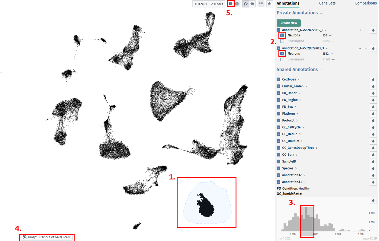
1. Lasso selection over the embedding plot in the center
2. Using the checkboxes of categorical annotations on the Annotations panel (see below)
3. Brushing over the histogram of numerical annotations on the Annotations or Gene Sets panel (see below)
4. The number of selected cells can be seen on the bottom left section of the plot area
5. After selecting, cells and their metadata can be further isolated with the Subset Cells button

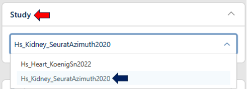
Study Selection

Users can select their study from this panel.

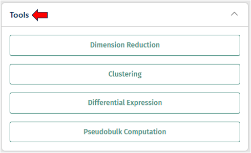
Tools panel

• The Tools panel allows users to perform various tasks on the loaded study
• Current options available include: Dimension Reduction, Clustering, Differential Expression, and Pseudobulk Computation

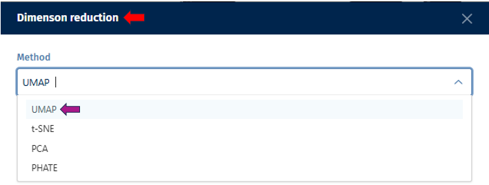
Dimension Reduction

The dimension reduction panel allows users to reduce the dimensionality of single-cell RNA sequencing (scRNA-seq) data for visualization and analysis. Users can select specific cells of interest by circling around them with the cursor.

By adjusting the options below, users can customize the dimension reduction process for their specific analysis goals.

1.Method: Choose a dimension reduction technique:

• UMAP (Uniform Manifold Approximation and Projection)

• tSNE (t-distributed Stochastic Neighbor Embedding)

• PCA (Principal Component Analysis)

• PHATE (Potential of Heat-diffusion for Affinity-based Transition Embedding)

2. Custom Name: Optionally, assign a custom name to the dimension reduction task for future reference.

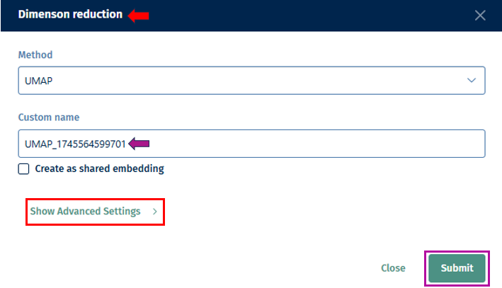
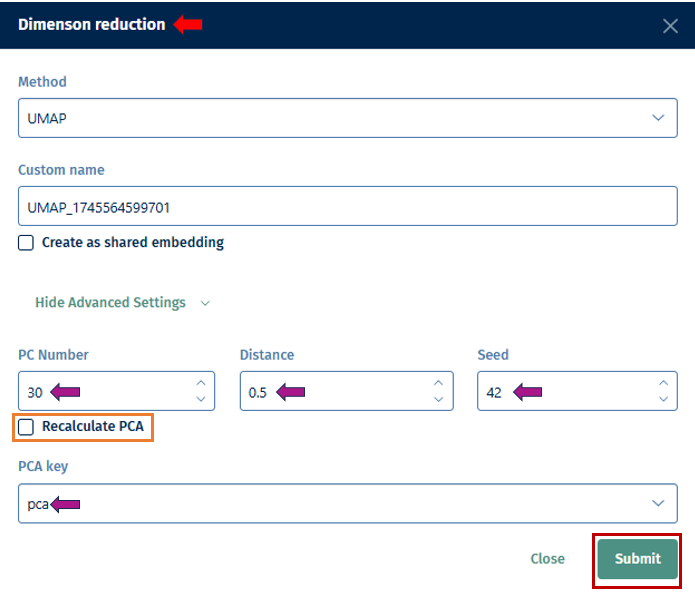
3. Show Advanced Settings: Depending on the technique, additional parameters can be set by enabling this option as described below.

   • PC Number: Define the number of Principal Components (PCs) to be retained in the dimension reduction process. This determines the level of detail preserved in the reduced-dimensional representation.

   • Distance: Set the minimum distance
     parameter for algorithms like t-distributed Stochastic Neighbor Embedding (t-SNE) or Uniform Manifold Approximation and Projection (UMAP). This parameter affects the clustering and separation of data points in the reduced space.

   • Seed: Specify the random seed or state to ensure reproducibility of the dimension reduction results. Using the same random state will produce the same results each time the analysis is run.

   • Recalculate PCA: Instead of using an existing PCA, recalculate and use it for the dimension reduction computation.

   • PCA key: Specify the key or feature of your dataset to be used for Principal Component Analysis (PCA). This could be gene expression values or any other relevant feature.

4. Submit: Initiate the dimension reduction process with the specified parameters. Once completed, you can explore the reduced-dimensional representation of your scRNA-seq data to gain insights into cell populations, gene expression patterns, and relationships between cells.

Clustering

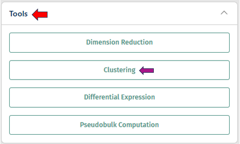
The Clustering panel provides options for annotating samples with metadata to facilitate downstream analysis and interpretation.

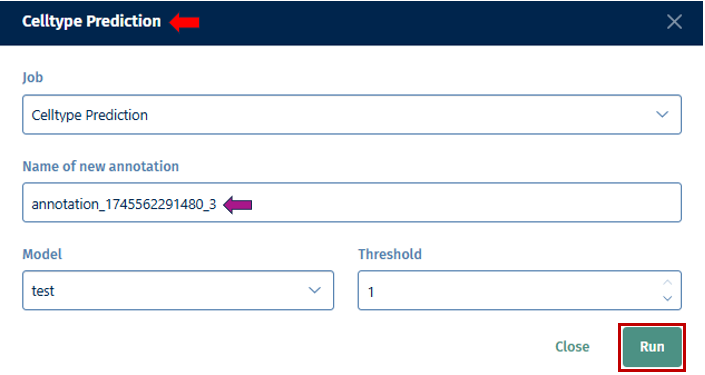
1. Job: Select an algorithm you want to use (e.g; Louvain, Leiden, Celltypist Prediction, Training, or Pseudotime) for clustering.

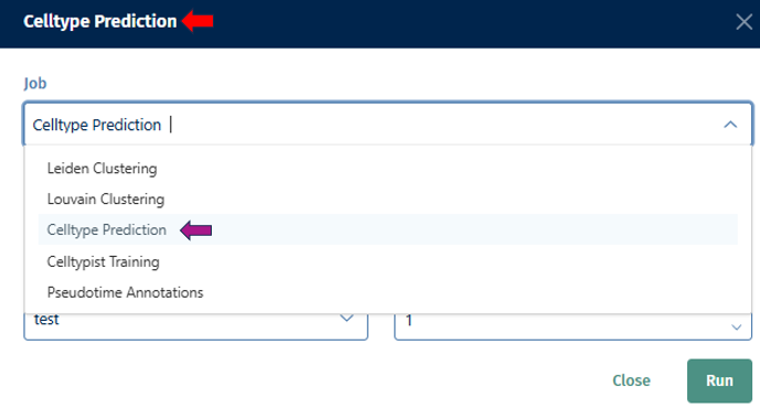
2. Name New Annotation: Assign a name for the new annotation that will be generated by the tool. This name helps you to identify and organize your annotations later.

3. Run: Once you’ve configured the parameters for the auto-annotation task, click “Run” to initiate the annotation process. The tool will analyze the data according to your specifications and generate the new annotation based on the selected parameters.

The interface allows for the complex selection of cells via selecting directly on the embedding, gene expression cutoffs, and based on categorical metadata attributes.

Differential Expression

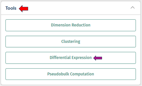
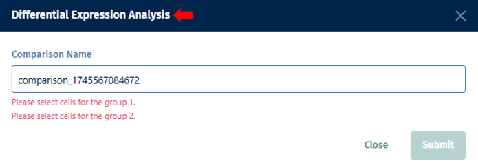
• Select the first group of cells and designate it as Population 1 by clicking on the button shown below.

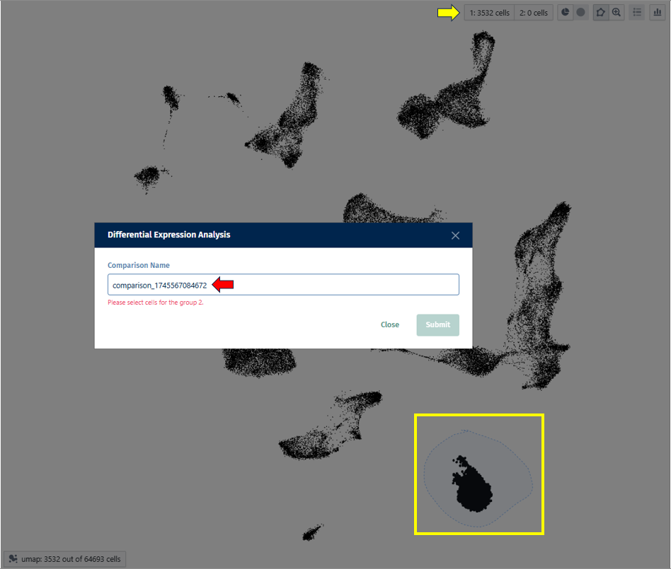
• Repeat for the second group (population 2).
• Click the “Differential Expression” button.
• Optionally, assign a custom name to the comparison.
• Click on the “Submit” button, to run your differential expression analysis.

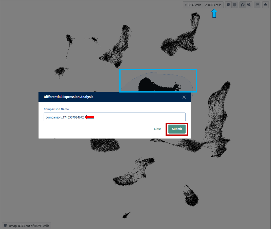
• Results appear in the “Comparisons” tab, on the right-hand column.

Pseudobulk Computation

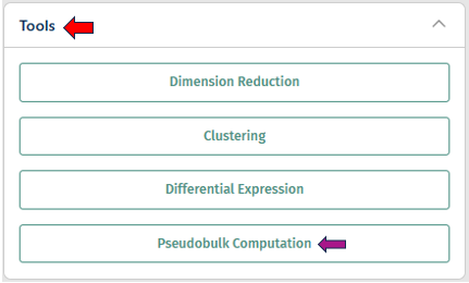
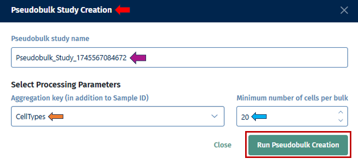
A pseudobulk study aggregates single-cell data into pseudobulk profiles, typically based on defined groups such as cell types or experimental conditions. This allows for bulk RNA-seq analysis techniques to be applied to scRNA-seq data, providing insights into gene expression patterns at a higher, more interpretable level.

Users can provide a name for their pseudobulk study in the “Pseudobulk study name” option. The “Aggregation key” is a parameter used in pseudobulk studies to specify how cells should be aggregated into pseudobulk profiles. In addition to the sample ID, which identifies individual cells, the aggregation key defines the grouping criteria for aggregation, such as cell type or other experimental conditions.

After configuring the parameters for the task, click “Run Pseudobulk Creation” to initiate the process.

Gene Selection panel

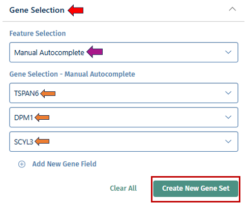
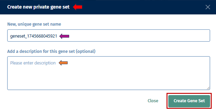
With the “Gene Selection” option, you have the ability to create your own set of genes used for more detailed exploration. Users can input their genes of interest by clicking the drop-down to create a custom gene set. This allows you to analyze the collective expression patterns of multiple genes simultaneously. Once done, click the “Create New Gene Set” button which will open a pop up box, where you can add a name for your geneset with a short description for your reference. After filling the information, click the “Create gene set” button to add it to the Gene set tab mentioned below.

Annotations tab

The Annotations tab contains all the cell metadata present in the study.

Private Annotations:

Private annotations consists of annotations that are only visible to the user who created them. Users can create new annotations using the below given features:

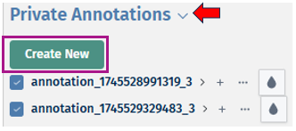
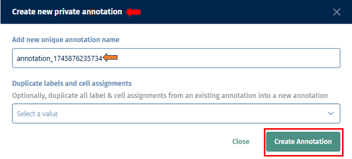
• Click on the Create New button. It will then open a Create new private annotation pop-up box in which you can add a new unique annotation name and also optionally duplicate all labels and cell assignments from an existing annotation to your new one. Then click on Create Annotation button to create your new annotation.

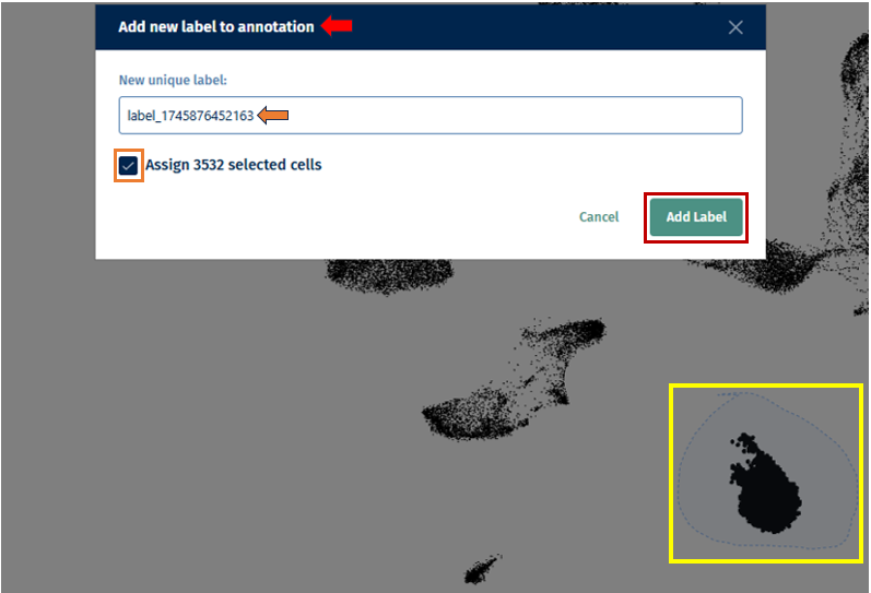
• After creating your new annotation, you can also add cell labels to it by clicking on the ‘+’ icon next to the annotation name. Before clicking on the icon, first lasso select your cells of interest to label. Then upon clicking on the ‘+’ icon, a pop-up box Add new label to annotation opens, in which you can add a new unique label name and click on the ’tick box’ to assign the selected cells. Then to confirm your selection, click on the Add label button.

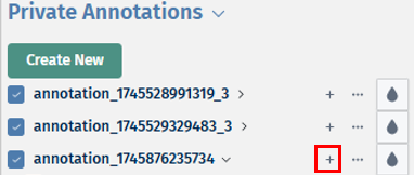
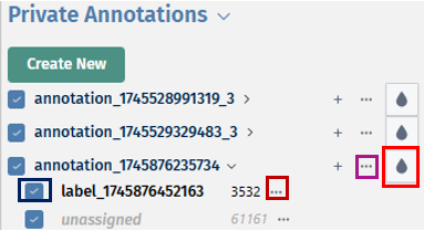
• By clicking on the dropdown button near your annotation name, you can view your added labels. The ’…’ icon near the annotation name provides you with options to ‘Edit this annotation’s name, Share annotation or Delete the annotation with all it’s assosciated informations’. With the help of the droplet icon, users can study their annotations along with their labels in different colours. The ’…’ icon near the label’s name provides you with options to ‘Relabel the label’s name to its common label name, Edit the label’s name or Delete it’.

Shared annotations:

Shared annotations can be accessed and viewed by other users who have access to the same dataset. This distinction allows for collaboration and sharing of annotations within research teams or across the scientific community.

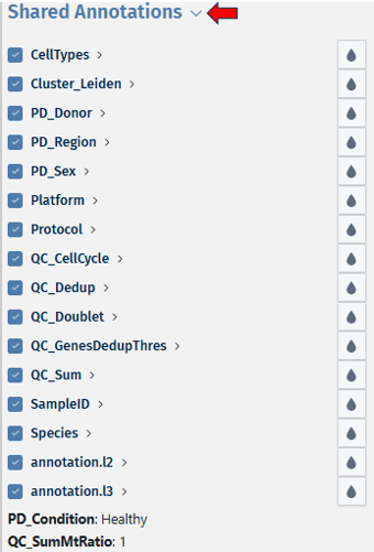
There are different options available to visualise the single cell data based on the following factors:

(i) “QC-sum” is shown by the percentile factors i.e. 1 means Top 20 percent and 5 mean last 20 percent, here 1 is best as it represent the cells with higher read counts

(ii) “QC-dedup” representing UMI counts as similar as QC-sum,

(iii) “QC-GenesDedupThres” showing number of genes detected by unique number of UMIs.

(iv) “QC-SumMtRatio”, representing mitochondrial to transcript ratio with respect to read counts. NOTE, here 5 represent the worst as it shows the highest mitochondrial-transcript ratio.

(v) “QC-SumDedupMtRation”, mitochondrial to trancript ratio with respect to UMI counts, similar to QC-SumMtRatio but with UMI counts. Further, a higher mitochondrial-to-transcript-ratio (typically > 0.7) means that the cells are either under stress or dying.

(vi) “QC-SeqCluster” represent whether two barcodes (cells) have barodes basepairs with 1 mismatch or indel; Yes means overlapping barcodes; No means unique barcodes.

(vii) “Cell-Cycle” (G1, G2M and S)

(viii) “Cluster” basically represents the clusters annotation.

Users can annotate and study the different cell groups based on these factors, by viewing them in various colour ranges with the help of the “Droplet icon” present near the respective annotation options.

Gene Sets tab

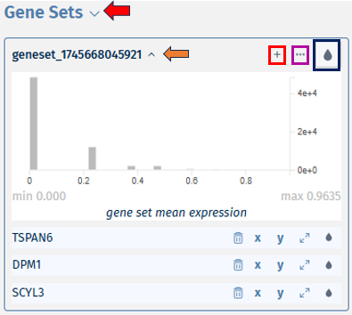
The Gene Sets tab allows analysis of group of genes. Users can create a geneset with the help of the “Gene selection”(mentioned above).

• By clicking on the dropdown near the geneset name, opens a bivariate plot. Comparison of the expression of multiple genes can be done using this bivariate plot, which display the relationship between the expression levels of two genes across single cells.

• The ‘+’ icon helps in adding more genes to the existing geneset. On clicking the icon, it opens a pop-up box ‘Add genes to geneset’ which consists of a ‘Genes to add’ dropdown. Users can then select their genes of interest to be added to the geneset from the list, and click on the ‘Add genes’ button.

• The ’…’ icon provides you with options to ‘Edit the geneset’s name and description, Share geneset or Delete the geneset’. The droplet icon helps in viewing it in different colour ranges for data analysis.

• Users also have the option to view the bivariate plots as scatter plots by clicking on the “x” and “y” buttons next to the gene names, allowing for a more detailed examination of the expression relationship between the selected genes. Users can click on ‘hide’ to minimise and ‘remove’ to close the scatter plot.

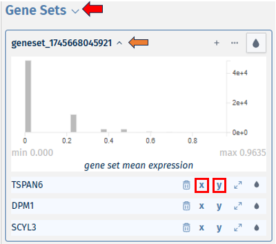
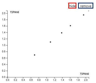
• The dustbin icon helps in deleting the particular gene from the geneset list. The expandable icon displays the expression level of the respective gene in the form of a bivariate plot. The droplet icon helps in viewing them in different colour ranges.

• Shared Gene Sets: This feature allows users to access and utilize predefined sets of genes that are shared among multiple users or datasets. You can similarly study individual gene from your shared gene set with the help of the options shown in previous examples.

Comparisons tab

The Comparisons tab displays all differential expression analyses you have submitted. Each comparison represents a differential expression job between two selected cell populations.

• Once the analysis is complete, selecting a comparison from the dropdown reveals a list of up-regulated (blue) and down-regulated (red) genes.

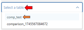
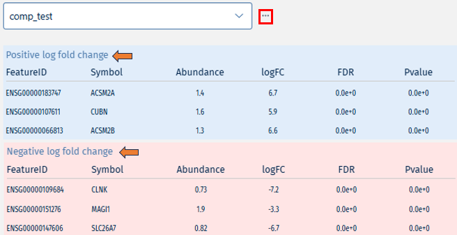
• The ’…’ icon next to each entry provides option to delete the comparison, allowing for easy management.