SampleQC

The Sample QC application is utilised to ensure sample quality, with an emphasis on RNA-seq and similar platforms. The application presents data supplied by the STAR aligner tool, Samtools, and the HTSeq package.

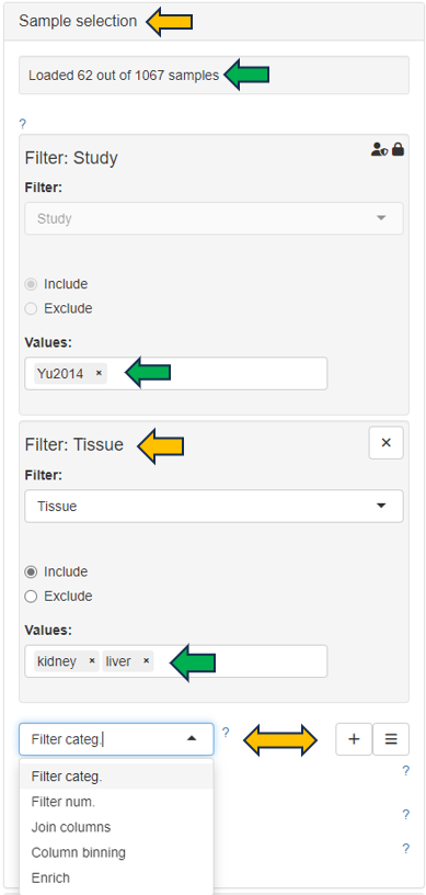
Samples can be selected through the “Sample selection” option located on the left side of the interface. The Sample Selector provides a variety of filters and other operations, called "Modifiers", that can be used to narrow down the samples selected from the entire catalogue of samples in your project to the ones you are interested in.​

1. Sample information shows you how many samples are selected and loaded according to the current settings.​

2. Filter Study is a “mandatory filter” to select and load your studies of interest. Please click on the field below “Values” to select the studies from a drop-down menu.​

3. Modifiers can be stacked additionally to narrow down the selected samples. For a more compact view, click on their titles to minimise them.​

4. Include or Exclude the specified values in or from your selection. ​

5. Additional modifiers can be selected from the drop-down menu and easily added by clicking on the + button. ​

   • Filter categ. can filter the samples according to categorical variables.​

   • Filter num. can filter the samples according to numerical variables.​

   • Join columns can combine two or more categorical variables into one.​

   • Column binning can devide samples into groups according to a specified numeric variable.​

   • Enrich can add additional information to your sample table, such as custom annotations. ​

6. Save, retrieve and share your selections are available by clicking on the “≡” button. ​

The detailed tables and figures for specific quality control aspects or platforms are available on the panels located on the right-hand side.

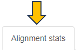
Alignment stats panel

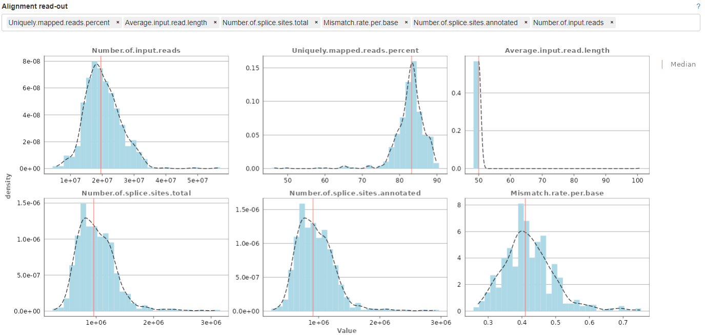
This panel displays histograms of alignment statistics, such as the number of input reads, uniquely mapped reads, average read length, number of splice sites, and the mismatch rate per base. The histograms show the distribution of these statistics for all selected samples while the values for the highlighted sample/files are indicated as colored line.

Read distribution panel

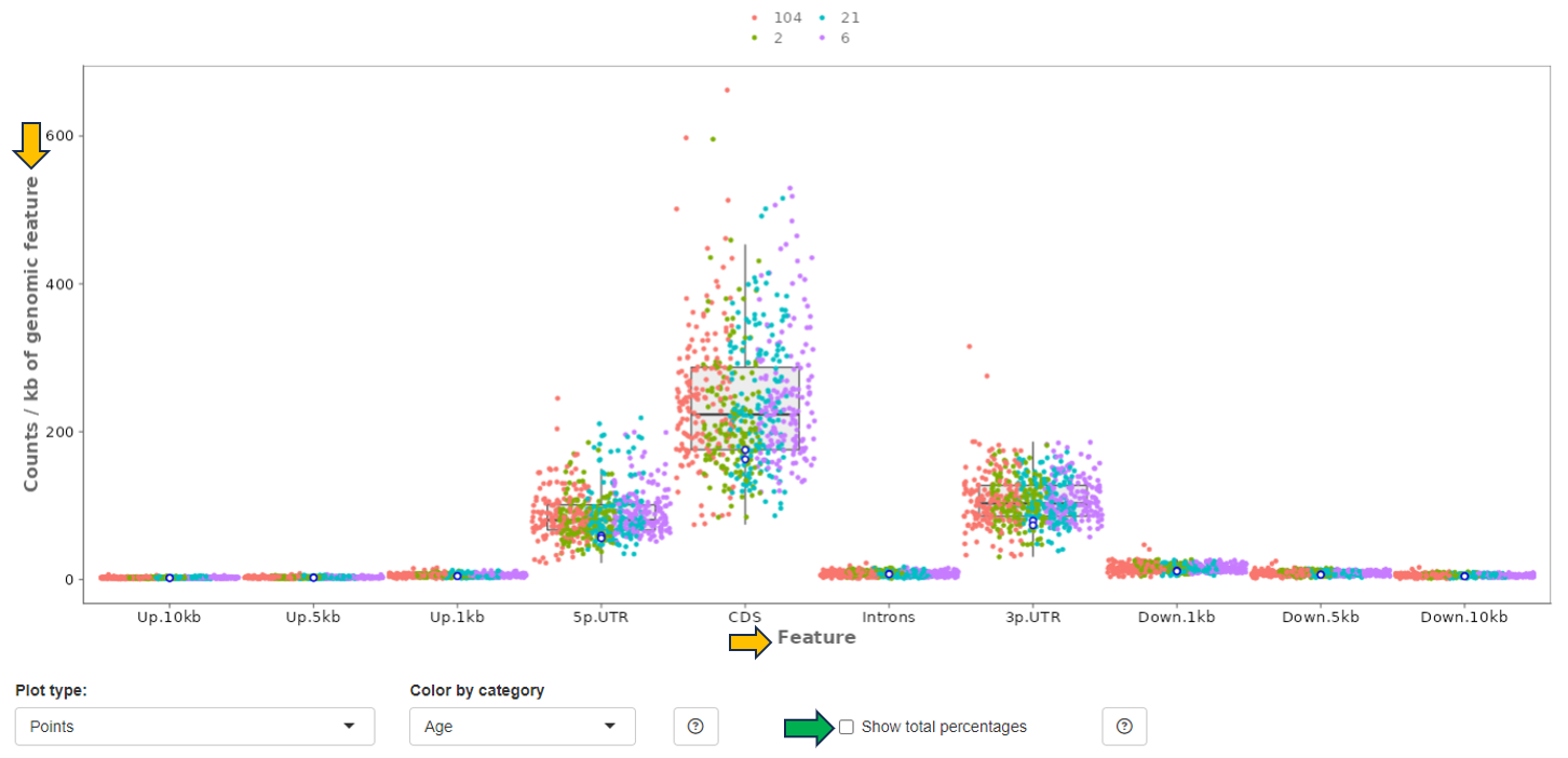
This panel provides a bar plot of the read distribution for the selected sample. The y-axis corresponds to counts which is mapped to different genomic features represented in the x-axis, e.g. CDS (coding sequences), Introns, 5’ and 3’ UTR, and remote up and down-stream regions. By default, the plot shows the distribution of counts normalized to the Kb of genomic features (in percentage). Check the checkbox “Show total percentages” to display the total counts distribution in percentages.

Gene body coverage panel

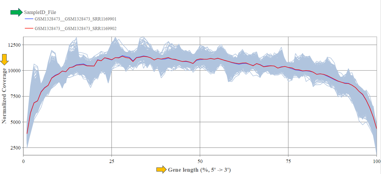
In this panel, the read coverage of genes is displayed. The y-axis displays the number of counts per gene sequence position (from 5’ to 3’) and the x-axis shows the gene position in percent of gene length. This figure may indicate issues with RNA degradation. The highlighted sample/files are shown as colored lines.

Biotype panel

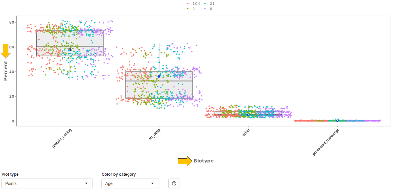
In this panel, the number of reads mapped to different gene biotypes, e.g. protein-coding genes, pseudogenes, or ribosomal RNA, are shown as bar diagram. The mean over all selected samples is displayed in contrast to the highlighted sample/files (encoded by distinct colors).

Mitochondrial panel

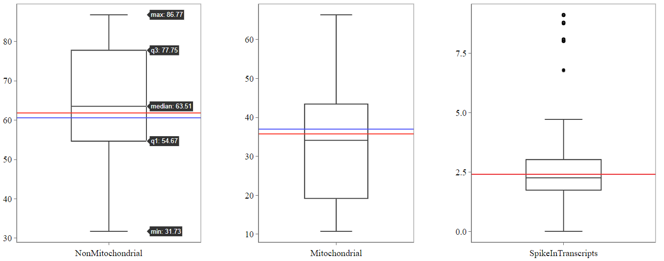
This panel contains boxplots of the percentage of reads mapped to mitochondrial genes, non-mitochondrial genes and spike-in transcripts. The boxplots show the distribution (e.g. median and quartiles) for all selected samples. The highlighted sample/files are depicted as colored lines.

Parameters panel

This panel shows the software versions and databases used for alignment and read counting of the selected samples. For optimal comparability, these parameters should be identical for all samples within a comparison.

The first table gives an overview and displays the number of samples which were processed with a specific combination of software versions and databases.

The second tables list the parameter for the individual samples.

Gene counts panel

This panel shows the mean and sum of counts for the selected study samples and genes. In addition, mean normalized expression values are displayed. If no genes are specified, the top 250 genes according to mean normalized values are selected.

Single cell RNA-Seq panel

In this panel, single cell RNA-Seq statistics and plots are displayed for the current sample divided into several subpanels. The number of shown barcodes or genes can be adjusted using the slider at the top of the panel, respectively.

Barcodes are usually sorted according to the sum of associated reads and plotted on the x-axis (barcodes with highest sum on the left-hand side). In the following, individual subpanels are described in more detail.

Stats: Table of general file specific statistics. The column “Detected” contains the number of sequenced reads or detected UMIs (Unique Molecular Identifiers identifying individual transcripts). “All” contains the corresponding reference number in order to calculate percentages (“Percent”). The rows correspond to the number of read assignments in the alignment (featureCounts output), the number of multimapping and uniquely mapped reads, the number of reads assigned to a feature (usually exon), unmapped reads, reads assigned to no feature, ambiguously mapping reads, reads not assigned due to low quality, the number of distinct UMIs after deduplication of reads, and the number of UMIs mapped to special spike-in sequences (e.g. phiX). Note that most phiX reads should have been removed during preprocessing.

Expressed Genes: Plot showing the number of genes (y-axis) above (greater or equal) a particular UMI count threshold (see legend). Default threshold, which is also used for cell filtering, corresponds to 2 UMIs. This plot is very useful when trying to estimate the number of sequenced cells vs noise.

Mt Genes: Plot showing the ratio of reads or UMIs per barcode assigned to mitochondrial genes.

Amplification (Barcodes): Plot displaying the summarized read or UMI counts per barcode. This can be used to estimate cell number or check PCR amplification issues.

Amplification (Genes): Plot showing the summarized read or UMI counts per gene. This can be used to check for a gene specific bias in amplification.

Amplification (Gene List): Plot showing the genes with the highest read count and their fraction of the total read count. This helps to identify over represented genes which might indicate a contamination. Mitochondrial and ribosomal protein coding genes are expected to have high counts.

Species Distribution: Plot displaying the distribution of species specific UMIs per barcode in mixed species control experiments. Each dot corresponds to one barcode. The sum of UMI counts associated with genes corresponding to the first species is depicted on the x-axis, the sum of UMI counts associated with the second species on the y-axis. This plot is shown only for mixed species samples and can be used to estimate contamination or cell doublets (more than one cell associated with the same barcode). Dot color corresponds to species classification. Note that the number of displayed barcodes can be adjusted using the slider at the top of the panel.

Barcodes: Summarized statistics for filtered barcodes (potential cells). The first table shows the number of filtered barcodes (“Cells”), the number and percentage of these barcodes matching the 10xgenomics whitelist (“Matching10x” and “Percent”, not used in the preprocessing), the number of reads for all filtered barcodes (“Reads”), the corresponding number of UMIs (“UMIs”), the ratio of reads vs UMIs for the filtered barcodes (“Amplification”), the ratio of reads for the filtered barcodes vs all barcode associated reads (“ReadCoverage”), and the ratio of UMIs for the filtered barcodes vs all barcode associated UMIs (“UMICoverage”) per sample (“Sample”). The second table contains count statistics for individual filtered barcodes. “Sum” corresponds to the sum of associated reads, “Dedup” to the number of deduplicated reads or UMIs, “Genes” to the number of genes above (greater or equal) the default UMI count threshold (usually 2). The third table shows the UMI count percentage/frequency of particular sequence motifs at particular barcode positions. Each position (column) sums up to 100 percent. This view can be used to identify position dependent preferences. The motif length can be adjusted interactively. The last table contains statistics on filtered barcodes with very similar sequences (one base mismatch/deletion/insertion). Too many rows may indicate issues with the barcode correction during preprocessing. “Counts” correspond to UMIs, “N” to the number of sequence neighbors (barcodes with similar sequence).

Cumulative Fraction: Cumulative fraction plot of the sorted barcodes. This plot shows the fraction of reads or UMIs associated with the first N barcodes (descending order of read sum). It can be useful to estimate the number of sequenced cells (barcodes representing most of the reads) or check the PCR amplification rate (reads vs UMIs) and issues with ambient RNA (no saturation of fraction). Note that the number of shown barcodes can be adjusted using the slider at the top of the panel.

Plate based RNA-Seq panel

This panel contains special QC statistics for selected (high-throughput) plateRNA-Seq samples splitted into separate panels. A plate is usually represented by two sequence files, the first one contains the (well specific) barcode and transcript UMI sequence and the second the actual cDNA read sequence which needs to be aligned to the genome. In the first step of preprocessing, unwanted sequences are filtered out and the corresponding barcodes are skipped, e.g. reads matching to phiX sequences, which were added by the sequencing provider. The other barcode sequences are then matched with the expected well barcodes and the corresponding reads are written out to single well/barcode specific files (the read sequence corresponds to the cDNA and the UMI is added to the read ID). This demultiplexing procedure also checks for barcode sequences with a single base mismatch or insertion/deletion compared to one of the reference barcodes and corrects this variant (assuming a PCR or sequencing error). The well specific sequence files are then aligned to the genome of interest and distinct UMIs are counted per barcode/well and gene (deduplication process). In the following, the individual subpanels are described in detail.

Files: Table showing statistics for all plate sequence files corresponding to the selected (reference) samples. “TotalReads” correspond to the number of reads detected in the input file, “Skipped Reads” to the number of reads which were filtered out (e.g. phiX), “Matching Reads” to the number of remaining reads whose barcode sequences match one of the reference barcodes exactly, “HammingReads” to the number of remaining reads which match assuming one base mismatch (Hamming distance 1), “SeqlevReads” to the number of remaining reads which match assuming a single insertion or deletion (sequence Levenshtein (edit) distance 1), “NotReads” to the number or remainig reads which could not be matched. “PercentDemux” is the percentage of the sum of “Matching Reads”, “HammingReads”, and “SeqlevReads” divided by “TotalReads”. This readout should ideally be in the range between 90 and 100 percent. “PercentSkipped” is the percentage of “Skipped Reads” divided by “TotalReads”, which should be below 5 percent.

Samples: Table showing the sum of UMI counts for selected samples. Columns in the middle of the table correspond to project factors/categories associated with multiple values for the selected samples. They can be used to filter the table for display. The column “Counts” corresponds to the final sum of deduplicated UMI counts per sample/barcode. The background colors match the respective values (from white for low counts to dark green for high counts). “Reads” represents the sum of demultiplexed reads for the corresponding barcodes and “Percent” the percentage (“Counts” vs “Reads”). Note that “Reads” also includes reads which could not be uniquely aligned to exon features. A low percentage may indicate issues with read alignment and/or library amplification. “ExactM” corresponds to the percentage of exactly matching barcode sequences compared to the sum of matched barcodes (exact match, one base mismatch, or one insertion/deletion). Ideally, this readout should be above 90 percent and comparable for all wells on a plate. By means of the “Grouping factors” selection box, only the selected factors/columns can be viewed before summarizing. This can be useful for reducing the table size or summarizing across multiple factor levels.

Plate: Table showing the color-coded UMI count sums per well in a plate layout. This plot is only shown in case well IDs are provided in the sample table (column “Well”). In case samples from multiple plates (see sample table “Plate” column) are selected, the plate IDs are added to the row part of the well IDs, resulting in stacked plate layouts.

Barcodes: Table of UMI count percentage/frequency of particular sequence motifs at particular barcode positions. Each position (column) sums up to 100 percent. This view can be used to identify position dependent barcode motifs. The motif length can be adjusted interactively.