New Comparison
The New Comparison app helps explore sample variability and configure differential analyses to identify differentially expressed genes or proteins between groups of samples (e.g. different treatments, tissues, or timepoints). Results and analysis parameters are stored in the Comparisons app.
On launch, the app displays the Studies Overview tab with an empty study table. No data is visible until at least one study is selected via the Sample Selection panel on the left.
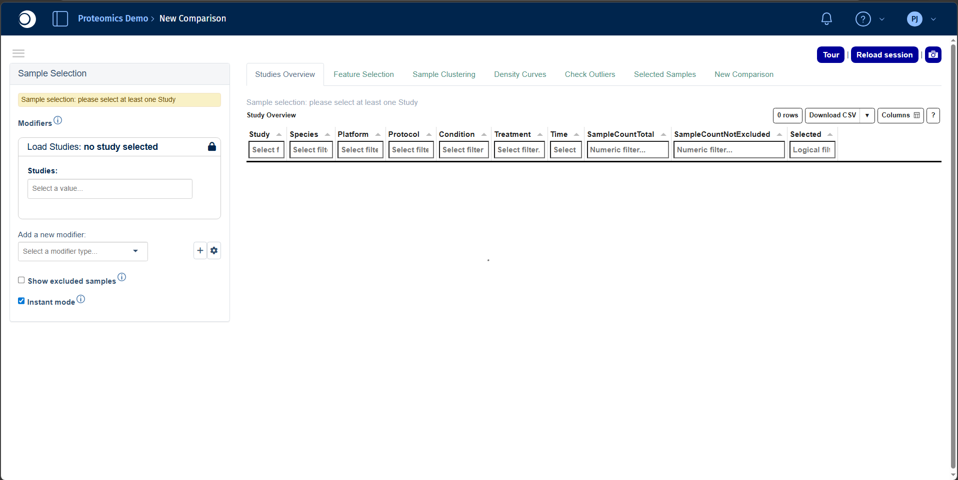
The interface consists of three main areas:
- Left sidebar: Sample Selection panel for controlling which samples and projects are loaded.
- Tab navigation: The app provides eight tabs visible across the top:
- Studies Overview tab
- Feature Selection tab
- Sample Clustering tab
- Density Curves tab
- Check Outliers tab
- Selected Samples tab
- New Comparison tab (will be retired with PanHunter v36)
- CG Calculation tab
- Main content area that updates dynamically based on the active tab and current sample selection.
Refer to the Sample Selector documentation for detailed instructions on selecting and filtering samples.
Studies Overview tab
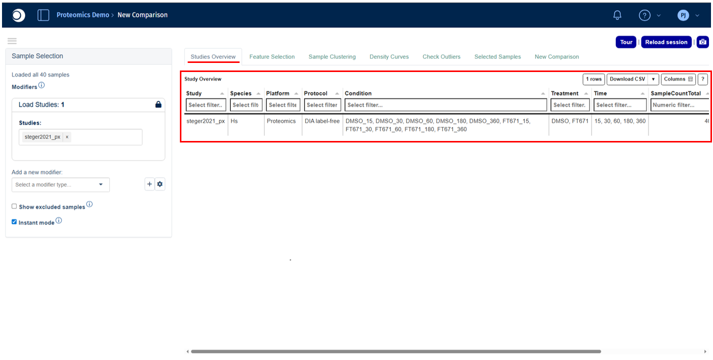
The Studies Overview tab displays a summary table of all available studies in the project, covering both technical platform information and sample metadata. It serves as the starting point for confirming which data is available before proceeding to analysis.
Refer to the Study Overview Statistics Table panel documentation for a detailed explanation of all available columns and filtering options.
Feature Selection tab
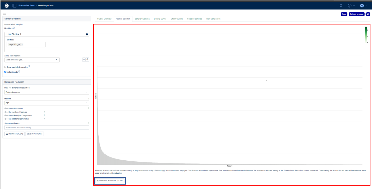
The Feature Selection tab visualizes and ranks feature variability across the selected samples. For each feature (e.g. gene, transcript, or protein), PanHunter calculates the variance of the selected data values and displays them in descending order. This allows identification of the most informative features for sample separation and downstream dimensionality reduction.
By default, the tab shows the top highly variable features used for dimension reduction. The plotted values depend on the selected data type and analysis mode. The feature list can be downloaded using the “Download feature list XLSX” option located below the plot. This will yield all features that were used for dimensionality reduction.
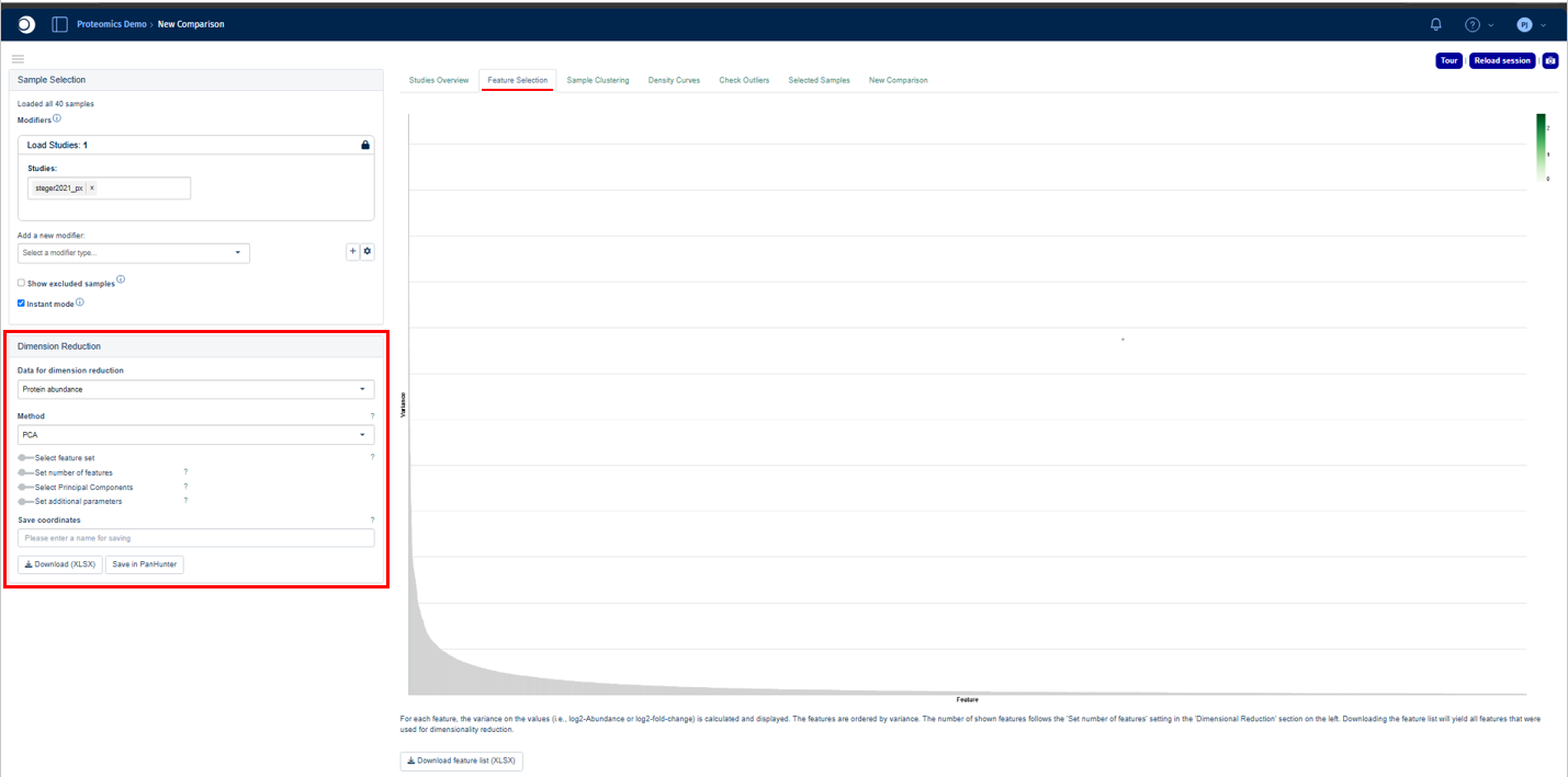
Users can explore and configure the plot using the options in the Dimension Reduction panel on the left sidebar.
Refer to the Feature Selection plot interpretation documentation for a detailed explanation of how to read the variance plot.
Sample Clustering tab
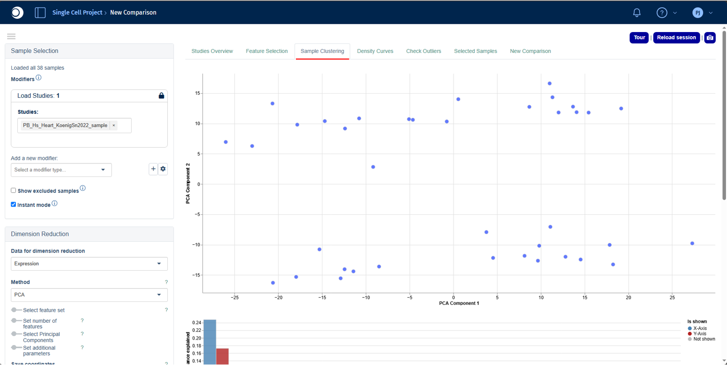
The Sample Clustering tab visualizes similarity between selected samples based on their feature expression or abundance profiles. Because these datasets are highly multidimensional, dimensionality reduction is applied to project the data into a two-dimensional space.
Refer to the Sample Clustering plot interpretation and Plot Options panel documentation for a detailed explanation on how to interpret and edit the plot, respectively.
Excluded samples are hidden by default and can be shown by enabling Show excluded samples in the Sample Selection panel.
Use the Dimension Reduction panel to configure the dimensionality reduction method, feature selection strategy, and analysis parameters. The Sample Annotations panel can be used to assign custom or clustering-derived labels to samples, while the Exploratory Analysis panel helps identify metadata variables and molecular features associated with the observed sample structure.
Density Curves tab
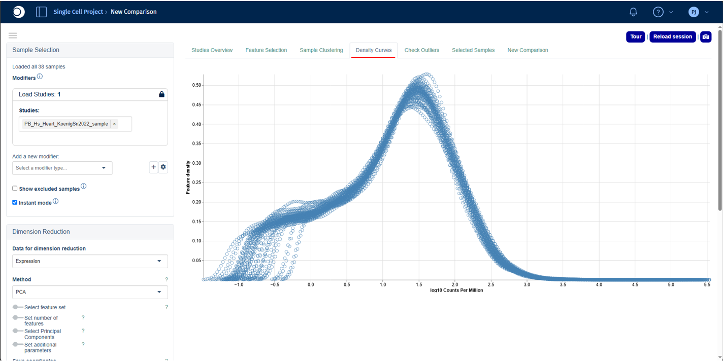
The Density Curves tab visualizes the distribution of feature expression or abundance values across the selected samples. Each curve represents a single sample, allowing rapid comparison of overall data distributions and helping identify potential differences in normalization, technical variation, batch effects, or biological variability.
Refer to the Density Curve plot interpretation documentation for a detailed explanation of how to interpret the density curves. Use the Plot Options panel to customize the appearance of the plot, including colors, symbols, labels, legends, and other display settings.
Check Outliers tab
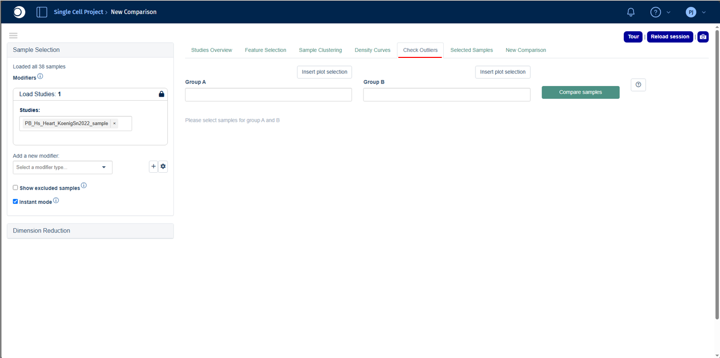
The Check Outliers tab provides a rapid exploratory comparison between two groups of samples. It is designed to help identify features (e.g. genes or proteins) that may be responsible for unusual clustering patterns or suspected outlier behavior observed elsewhere in the app.
This tab is particularly useful when samples appear separated from the main cluster in the Sample Clustering plot or show atypical distributions in the Density Curves tab.
Comparing sample groups
To perform an outlier comparison:
- Select the suspected outlier sample(s) in the Sample Clustering plot.
- Click Insert plot selection to add the selected samples to Group A.
- Select the reference samples and insert them into Group B.
- Click Compare Samples to run the analysis.
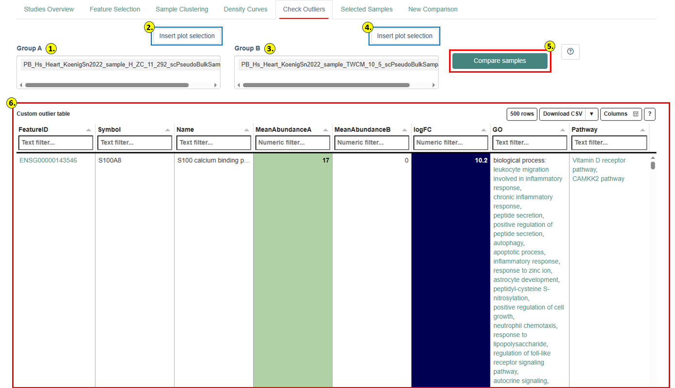
Custom Outlier Table
Results are displayed in the Custom Outlier Table, which lists features with the largest differences between the two groups. For each feature, the table shows the Feature ID, Symbol, Name, Mean log-intensity A, Mean log-intensity B, and logFC (logarithmic fold change). The table is color-coded for rapid identification of enriched or depleted features.
Features are automatically filtered to retain only those with mean abundance above a minimum threshold in at least one group and an absolute log fold-change above a minimum cutoff. The table shows the top features ranked by absolute fold change.
Identified features may help explain outlier behavior and can inform decisions on whether a sample should be retained or excluded from downstream analyses. Possible causes include pathway activation, treatment-specific responses, tissue contamination, technical artifacts, or batch effects.
Refer to the Study Overview Statistics Table panel documentation for a detailed explanation of all available columns and filtering options.
Important: The Check Outliers tab performs a rapid exploratory comparison only. No statistical significance testing or p-value calculation is performed. For statistically rigorous analyses, use the New Comparison tab.
Selected Samples tab
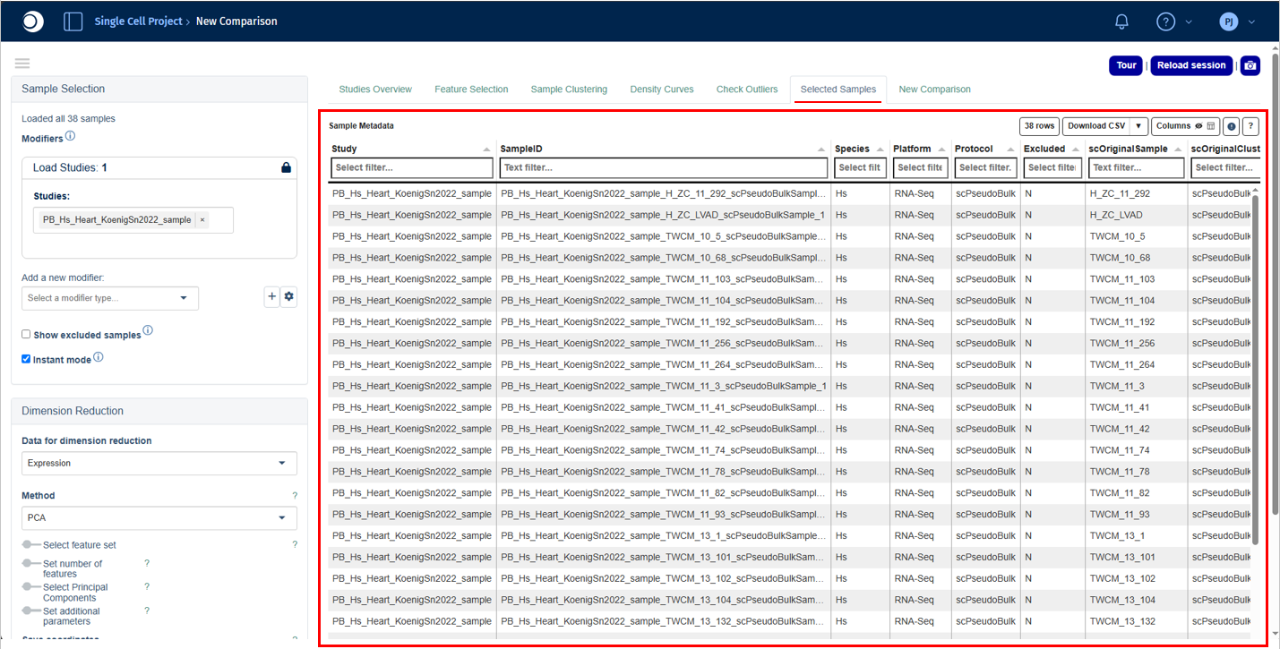
The Selected Samples tab provides a detailed overview of all samples currently included in the analysis. It is the recommended place to review sample metadata, experimental annotations, and quality-related information before proceeding with downstream analyses.
Sample Metadata table
The Sample Metadata table displays one row per sample with all associated metadata attributes, including Study, SampleID, Species, Platform, Protocol, Status, Treatment, Condition, batch identifiers, and platform-specific metrics such as precursor counts or injection order.
This tab is particularly useful for confirming correct sample selection, verifying metadata consistency, checking treatment and condition assignments, and identifying technical confounders such as batch effects.
For some data types, additional platform-specific metadata or preprocessing parameters are displayed below the main table (e.g. alignment and reference genome details for transcriptomics studies, or acquisition parameters for proteomics). These parameters should generally be consistent across samples within a study to ensure reliable comparisons.
Refer to the Study Overview Statistics Table panel documentation for a detailed explanation of all available columns and filtering options.
New Comparison tab
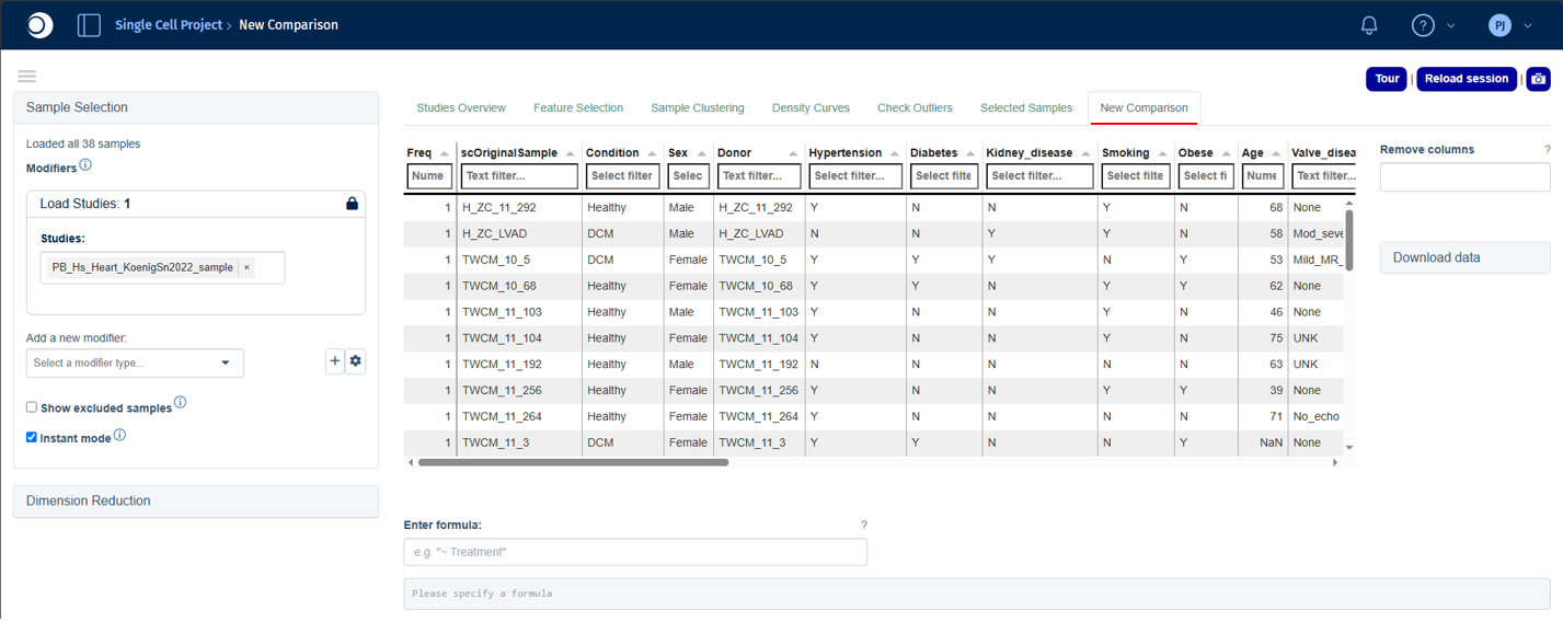
Important: Starting with PanHunter v36, the New Comparison tab will be retired. Use the CG Calculation tab instead: it covers the same single-comparison workflow and additionally lets you generate and submit many comparisons at once.
The New Comparison tab is used to configure and run differential analyses between selected sample groups. It provides a flexible interface for defining comparison designs, selecting statistical methods, applying feature filters, and generating results for downstream interpretation.
The workflow consists of four steps:
- review the sample group distribution,
- define the comparison formula,
- configure contrast and
- filtering options, and run the analysis.
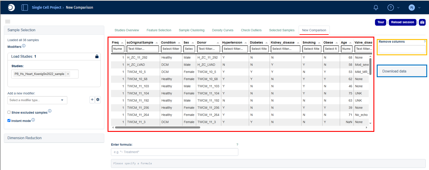
At the top of the tab, PanHunter displays a summary table showing the distribution of samples across available metadata categories. The Freq column shows the number of samples in each category combination. Use the Remove columns option to focus on relevant factors, and Download data to export the table and associated abundance data.
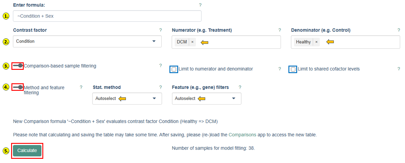
- Defining the comparison formula: The comparison design is specified in the Enter formula field.
Important: Formula names are case-sensitive and must exactly match the metadata column names shown in the sample table.
For a single-factor comparison, use a tilde (~) followed by the factor name:
~Condition
For multi-factor comparisons, combine factors with the + operator:
~Condition + Sex
Multi-factor designs allow PanHunter to account for additional sources of variation and reduce confounding effects during statistical analysis.
-
Selecting the contrast: After entering a valid formula, three additional fields appear.
- Contrast factor specifies which variable from the formula is being tested.
- Numerator defines the group of interest;
- Denominator defines the reference or control group.
For example, setting Condition as the contrast factor with DCM as numerator and Healthy as denominator evaluates differential abundance between those two condition groups. PanHunter displays a summary statement confirming the exact comparison before calculation.
-
Comparison-based sample filtering: When Limit to numerator and denominator is enabled, only samples in the selected numerator and denominator groups are included in model fitting. Limit to shared cofactor levels can be enabled for multi-factor designs, retaining only samples with cofactor levels shared between both groups making it useful for ensuring balanced comparisons.
-
Method and feature filtering:
- Stat. method: selects the statistical framework. DESeq2 is used for count-based transcriptomics data; limma is used for proteomics and continuous abundance datasets. PanHunter automatically selects the appropriate default.
- Feature filters: controls pre-filtering of features before model fitting. Options include automatic, model-based, or no filtering. Filtering removes low-signal features and improves statistical robustness.
- Lognorm intensity threshold: specifies the minimum normalized abundance required for a feature to be retained, evaluated across at least the specified fraction of samples for at least one contrast level.
- Sample fraction: defines the minimum fraction of samples that must satisfy the abundance threshold. The default for proteomics studies is typically 0.6667 (two-thirds of samples).
-
Running the comparison:
- After configuring all settings, click Calculate to start the analysis. PanHunter displays the number of samples that will be included in model fitting so you can verify the comparison is adequately powered before proceeding. Depending on dataset size and complexity, the calculation may take several minutes.
- After completion, the generated comparison can be saved and accessed through the Comparisons app for further exploration, including interactive result tables, volcano plots, MA plots, and pathway enrichment analyses.
- For detailed information on the underlying statistical methods, see the Differential Expression Calculation documentation.
CG Calculation tab
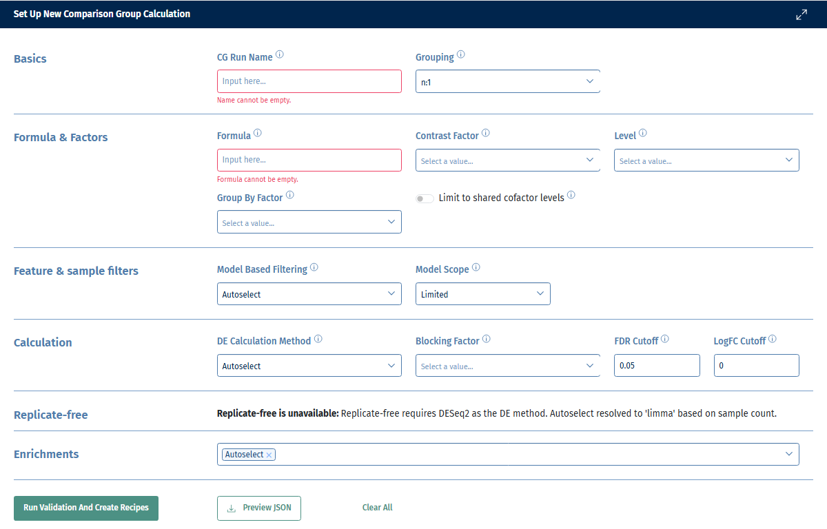
The CG Calculation tab lets you configure, validate, and submit a comparison group (CG) calculation: a single named run that can generate and compute many differential expression comparisons at once (for example, every pairwise comparison across the levels of a factor), instead of calculating one comparison at a time as in the New Comparison tab. The tab is organized into three sections, displayed one below the other: Set Up, Validation Results, and Job Overview.
Set Up
The Set Up section collects everything needed to build the calculation, grouped into seven parts:
- Basics:
- Give the comparison group a unique name. If the name matches an existing comparison group, an override option appears, letting you replace it; otherwise the name must be unique.
- Choose the grouping mode, which determines how comparisons are generated from your contrast factor:
- n:1 – compare each level of the contrast factor against one or more selected (control) levels.
- n:m - useful when more than 1 control is part of the study design. Each level of the contrast factor that is not itself a control level is compared to each (control) level separately. n:m requires at least two levels to be selected - if you do not want that use n:1 grouping instead.
- all:all – automatically generates every pairwise comparison across all levels of the contrast factor.
- fixed – Control samples are grouped into denominator sub-groups defined by the Denominator Scope factors (a strict subset of the Group By Factor columns).
- time-series – compares samples across an ordered sequence of time points, using an Offset to define how many steps apart two compared time points are (e.g. an offset of 1 compares each time point to the previous one); specific time points can be excluded via Exclude Levels, and their order set via Order. For more detailed explanations of the groupings please refer also to the extensive user guide.
- Formula & Factors: enter the comparison Formula (same syntax as the New Comparison tab, e.g.
~Condition + Sexor with no intercept~0+Condition +Sex) and pick the Contrast Factor to test. Depending on the grouping mode, additional fields appear: Level (the denominator level to include), Group By Factor (columns used to split the comparison into subgroups, e.g. per batch or per cell type), Denominator Scope, Exclude Levels, Order, and Offset as described above. Enable Limit to shared cofactor levels to restrict each generated comparison to samples whose cofactor levels are shared between the groups being compared. - Feature & sample filters: choose the feature filtering strategy (Autoselect, None, or Custom values). For Custom values, set the count/intensity threshold (labeled Count Threshold for most platforms, Intensity Threshold for proteomics) and the minimum sample fraction required to pass it. The default Count Threshold for transcriptomics is 5; the default Intensity Threshold for proteomics is 0. For the sample ratio the defaults are 0.2 and 0.6667 respectively. The Model Scope field lets you choose either Limited or Full: with Full, all samples are used for model building; with Limited, only the samples in the numerator and denominator are used.
- Calculation: choose the DE Calculation Method (Autoselect, DESeq2, or Limma); a Blocking Factor column appears when Limma is used. Set the FDR cutoff and LogFC cutoff for significance; both are pre-filled with platform-specific defaults and can be edited.
- Replicate-free: an optional mode for datasets without biological replicates. It is only available when the grouping mode is not fixed and the effective DE method is DESeq2; the UI explains why it is unavailable otherwise. When enabled, choose the Plate Column and Unique Identifier Column, and optionally set Independent Hypothesis Weighting to a Custom alpha.
- Base Enrichments: select which enrichment collections to run alongside the comparison, or leave this on Autoselect. See the Enrichment Analysis documentation for details on the underlying method.
- Signature Enrichments: signature enrichments are limited to 2 signature collections per comparison group due to the large memory consumption.
When ready, click Run Validation and Create Recipes to validate your configuration and build the individual comparisons (called recipes) to be reviewed in the Validation Results section below. Use Preview JSON at any time to inspect the underlying configuration that will be submitted. The Json can also be used to run in the backend and leads to the same results (unless recipes are filtered - see below - that is not reflected in the json), or use Clear All to reset every field on this page back to its defaults.
Validation Results
After clicking Run Validation and Create Recipes, this section shows the outcome, split across three tabs:
- Errors – problems that prevent the calculation from running (e.g. missing samples for a contrast); these must be resolved before you can submit.
- Warnings – issues that do not block submission but are worth reviewing (e.g. a sample-selector rule that could not be translated exactly, in which case the selected sample IDs are used as a safety net).
- Info – additional notes about how the calculation was built.
Each message is labeled with its origin (e.g. a specific recipe or layer) to help you locate the relevant setting above.
Below the messages, the created recipes table lists every individual comparison that will be computed, with its study, species, platform, contrast factor and levels, numerator/denominator sample counts (hover over a count to see the exact sample IDs), formula, DE method, model-based filter, and LogFC cutoff. For the n:1, n:m, and all:all grouping modes, each row has a checkbox so you can deselect comparisons you don’t want to submit; this selection only affects what gets submitted to SLURM and does not change the JSON preview.
Important: If you choose the full model scope then excluding recipes still uses the full Sample Table for model building. If you instead use the Sample Selector to filter the Sample Table to get to the same recipes, the filtered Sample Table is used for model building. That is expected, but needs to be kept in mind when using the full model scope with filtered sample or recipe table.
Important: If results are stale relative to your current setup (i.e. you changed a Set Up field after the last validation), this section asks you to re-run validation before showing messages or recipes again.
Once validation succeeds and at least one recipe is included, click Submit Calculation to SLURM to queue the calculation for computation. The button is disabled until there are valid, selected recipes, and again after a successful submission until you change the configuration.
Job Overview
This section tracks the SLURM (compute cluster) jobs belonging to your submitted runs. Use the Run dropdown to select a submitted run and see:
- A summary line with the run’s submit, start, and finish times.
- A table of its jobs, each with an ID, name, status (Pending, Running, Suspended, Cancelled, Finished, or Failure), nodes, CPUs, and memory. The list refreshes automatically while jobs are active.
- A Show Log button per job, opening its output log in a popup for troubleshooting.
- A Failed comparisons panel, listing any individual comparisons that failed during computation along with their error message, so you know exactly which ones to investigate or re-run.
If no calculation has been submitted yet, this section prompts you to submit one from the Validation Results section first.