This is the multi-page printable view of this section. Click here to print.
Data
- 1: Data Quality Control
- 1.1: Quality Control for Bulk RNA-Seq data
- 1.1.1: Starting quality control
- 1.1.2: Deeper look into SampleQC
- 1.1.3: QC clustering
- 1.1.4: Finalizing the Quality Control
- 2: Data Administration
- 2.1: PanHunter Preprocessing
- 2.1.1: Reference genomes
- 2.2: Studies overview
- 2.3: Data upload
- 2.4: Updating data
- 2.5: Deleting studies
1 - Data Quality Control
1.1 - Quality Control for Bulk RNA-Seq data
1.1.1 - Starting quality control
General assesement in the Project Overview
In the project overview app, you can check the general parameters for your study, such as the sample size or if the important variables are visible in the details tab.
Investigating Alignment statistics
For further statistics about the data integration we need to go into the ‘Sample QC’ app. First, we are presented with the Alignment statistics tab, showing different histograms for quality parameters.
Number of input reads
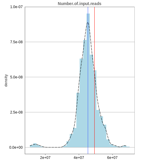
The first histogram is concerned with the number of input reads. While the blue vertical bar shows the median, the red bar shows the position of the current sample selected. A low number of reads can correspond to problematic data, while the definition of “low number” is sometimes subjective and numbers might depend on tissue type or species. Panhunter uses different color codes ranging from white to green to show low to high number of reads in the table below.
While absolute reads may be hard to distinguish by, big jumps should be investigated closely. While most of the data in the picture has 30-60 million reads, there are samples that have half or even less of the input reads. Taking these samples out should yield more homogeneous data which are more meaningful for further analysis.
Unique mapping
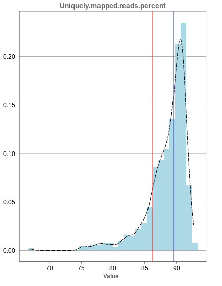
The general plot structure is similar to that of the number of input reads, such that we still want to detect outliers in the histogram. Because non-unique mappings of the input reads are not considered as reads in Panhunter, having a high percentage of uniquely mapped reads is very important.
While the displayed percentage above 85% is good for most samples, there is one with under 70% that should be omitted from the data. This also depends on the type of tissue that was used, such that the given number of 85% is considered meaningful for blood, but when using muscle cells, there might be much more lower numbers.
Mapping to multiple locations
While some reads are uniquely mapped, there is also the case of reads that are not mapped at all and reads that are mapped to multiple locations. As said before, these are not considered in the preprocessing of Panhunter, and only uniquely mapped reads are relevant for the count matrices.
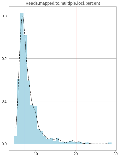
The remaining percentage of reads should largely be composed of multiple mapped reads, i.e. the number of reads that map to no location should be small.
1.1.2 - Deeper look into SampleQC
There are various other tabs in SampleQC, that are relevant for BulkRNA data.
Read distribution
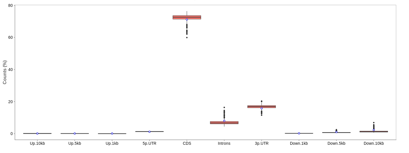
First of all, the box for total percentages should be ticked in the bottom for better comparison.
Ideally, the percentage of counts mapping to the highest should be CDS which stands for coding DNA sequence, relating to the region that codes for protein.
Also important is that up- and downstream are not mapped often.
Gene body coverage
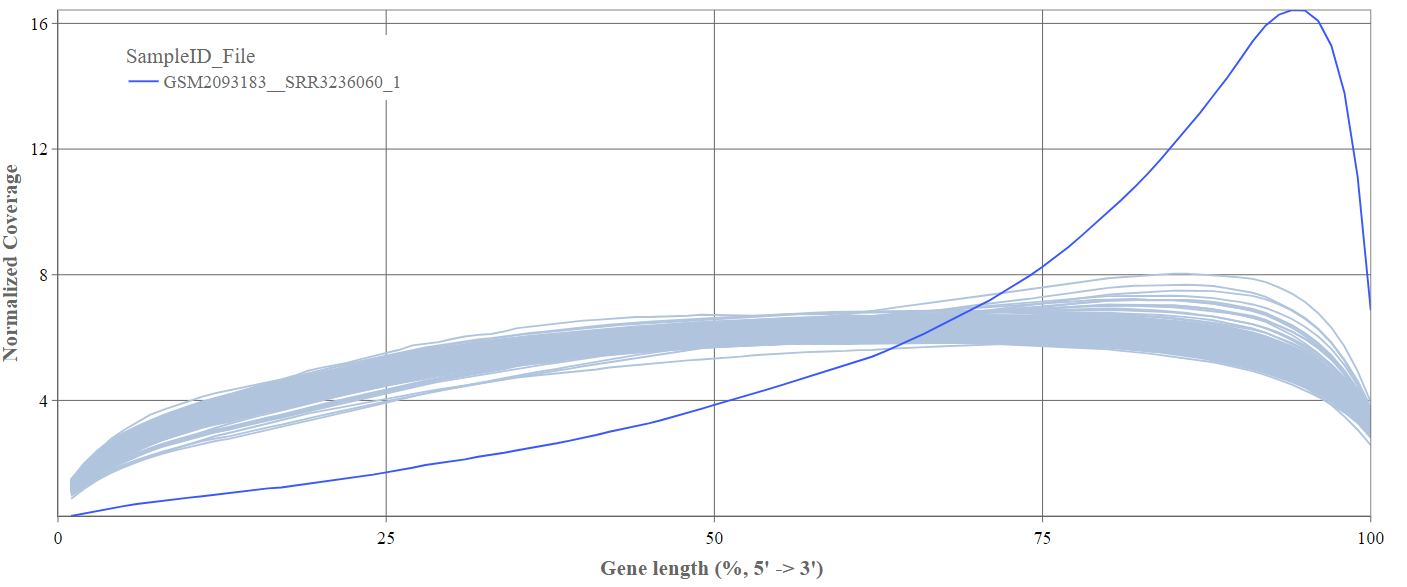
We can see the normalized coverage. The samples gene body coverages should be close to one another and should form a homogeneous band and, in BulkRNA-Seq, should be spanning quite ‘uniform’ over the gene length going down at the start and endpoints. Please note that evoenthouth this QC section is called gene body coverage we effectively measure the coverage along the RNA transcripts corresponding to the gene.
The sample colored in blue shows very untypical behaviour and is advised to be excluded.
Biotype
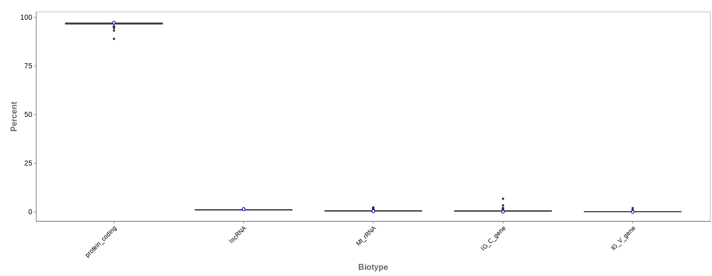
The biotype (that is functional types of the genes to which reads are mapped) can be used for quality control. The protein_coding should be the highest and not far away from 100%. We can also see in our example that there we have IgC and IGv genes for tuberculosis data, which seems reasonable because they are relevant for the immune/antibody system of humans.
Mitochondrial
Usually, the proportion of transcripts mapping to mitochondrial genes should be low. If there is phenomenons such as cell death, the amount of mitochondrial transcripts increases and we might infer a lower quality for the data.
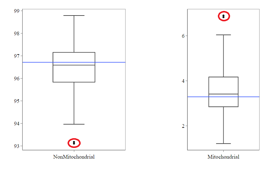
In our example, it may be useful to take out the two circled samples because they are clear outliers from the rest of the data.
Genes
An additional evaluation can be done by looking into the Genes tab, checking which genes are counted the most. The interpretation of this analysis is experiment specific and requires knowledge of the biological system that is investigated.
1.1.3 - QC clustering
The quality of the data can also be inferred from gene expression profiles represented via dimension reduction methods. Suitable methods in Panhunter are PCA, t-SNE and UMAP. The ‘New Comparisons’ app should be used in the following.
Clustering by sex
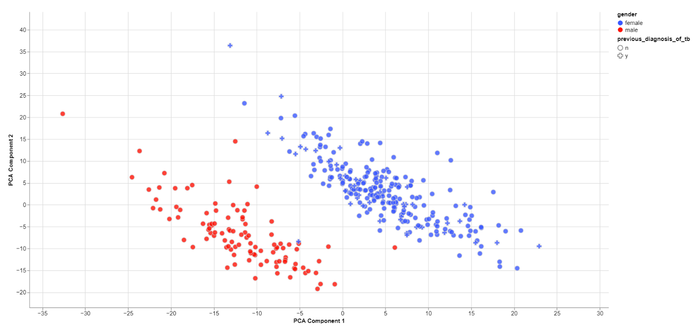
The biological sex should always be one of the greatest disparities between data points because an entire chromosome is different. Thus, there may be reason to exclude samples that are truly different from the rest of their group. However, some studies list gender which should not be confused with the biological sex.
What can also be inferred from the plot is that, in this data set, only females have been diagonsed with tuberculosis before, leading to a dependence between gender and previous_diagnosis_of_tb. These relationships are very important because correlation explained by the previous diagnosis can in some cases be completely explained by the gender/sex association.
PCA features
The categorical and numerical variables that are responsible for the variance in the data can be calculated with the buttons shown below in the picture.
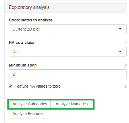
⚠️ Keep in mind that the default is to analyze only the current 2D plot of the dimensional reduction and may vary even by method (PCA,t-SNE, UMAP).
Check outliers
Even when there is no gender/sex variable present, there might be clear clustering. When comparing two groups, one can use the check outliers tab after selecting the groups, to look at up and downregulated genes and infer information from the results.
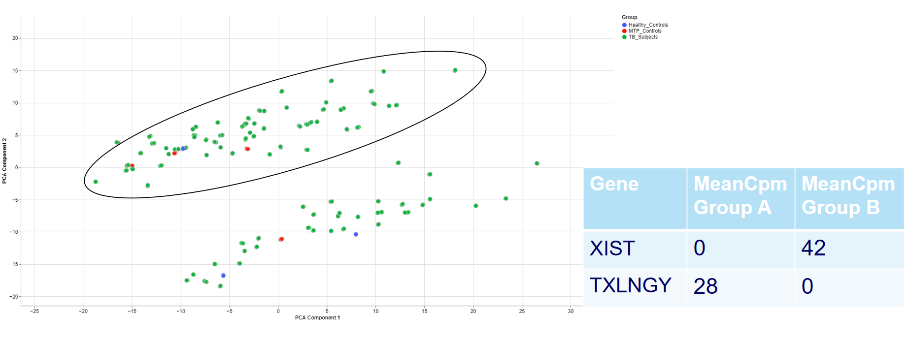
For example, the two groups are clustering completely different in the PCA plot. Even when there is no labeling variable, the comparison shows that certain genes are more present in the groups. Because the presented genes belong to the inactive X chromosome and the Y chromosome, we can infer that there are males and females in the data.
This is important for quality control because of the large influence of the biological sex which might otherwise be neglected.
Clustering of other features
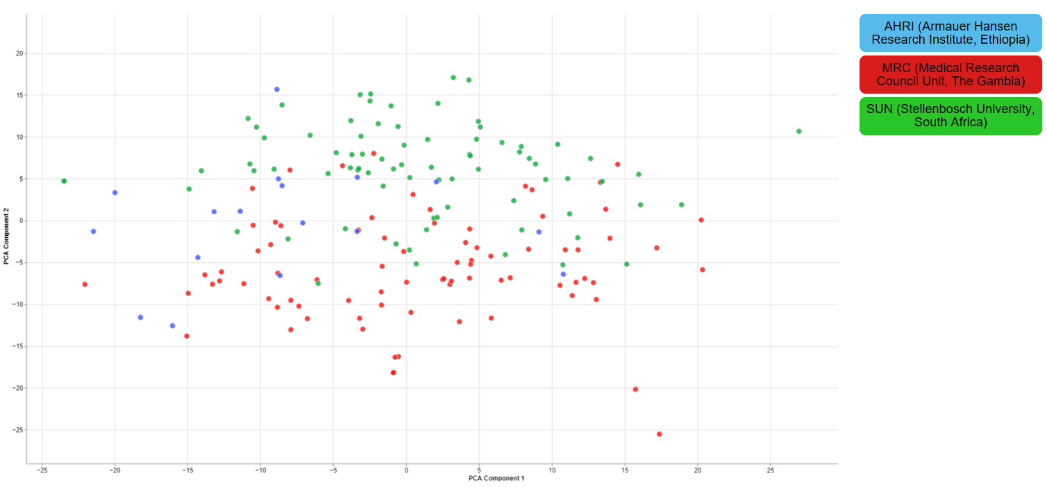
For one of the studies, different sites were used to collect blood samples from participants. This inevitable lead to differences that have to be accounted for and are thus important for the quality of the data.
1.1.4 - Finalizing the Quality Control
There are still various things that can be done to investigate the quality of the data but just a few final thoughts are mentioned down below.
New comparisons
As outlook, one can fit a group comparison in the app ‘New comparisons’, tab ‘New comparison’ with relevant groups, such as TB_subjects against control. If important genes are up/downregulated, then this is another sanity check that can be done.

Reporting on the quality
If there are multiple studies, one could present as follows:
- general setup of the study, things that are noticeable immediately (samples missing)
- general QC stats
- clustering
- variables that are relevant and should be/should not be
- New comparison between important groups, i.e. treatment vs control
- short summary of the study, the QC and important conclusions
- general setup of the next study
- comparison of all studies
- Slide with table: study | sample | reason to take out
2 - Data Administration
This section explains to the users how to perform the following data management activities:
- Overview of available studies and their upload status
- Uploading, updating and deleting data
2.1 - PanHunter Preprocessing
2.1.1 - Reference genomes
For the following species reference genomes are available in PanHunter: TO-DO give list
For model species such as mouse and human we maintain several reference genomes. If you would like to know which ensemble version is the latest in the respective release please see our changelog. The reference genome consists of a fasta file that represents the actual DNA strands and an annotation file (gtf file) that contains the positional information of every gene in the genome/fasta file.
For the human reference genome the soft masked (sm) primary assembly is used and this is then extended at Evotec with custom spike-in sequences. Soft-masked means that the nucleotides for repeat stretches are converted to lower-case. Repeats can also be masked (rm), then repeat associated nucleotides are converted to N's. The primary assembly tracks a single unbranched path through the genome. In other words there is only a single base per position and the so called haplotype (alternative base calls) are not included. Toplevel fasta files also include alternative base calls/ haplotype information.
One of the spike-ins, that the soft-masked primary assembly is extended with at Evotec, is PhiX174. PhiX174 is often used in illumina sequencing runs to increase the library quality or balance the GC content (See Phix Illumina version3 - product by illumina). Please note that the reads for PhiX should not be assigned to the fastQ files because there is no index read attached to the PhiX transcripts. Sometimes these reads do get erroneously assigned to a fastQ file due to index read bleeding (the index of a closeby cluster on the flowcell is interpreted as the index of PhiX). Barcode hopping could the other reason for an erronous assignment, this happens when indices break of and reattach within the multiplexed libraries.
The fasta file and gtf annotation contain spike in information for PhiX and for EGFP as well as for 92 ERCC (External RNA Controls Consortium) spike ins that are used to control for variation in RNA sequencing experiments.
2.2 - Studies overview
Overview of all available studies in the project
Newly created project
The Data tab lists all studies of the project and indicates the state of samples for each study. Initially, for the newly created project, there will no studies listed:
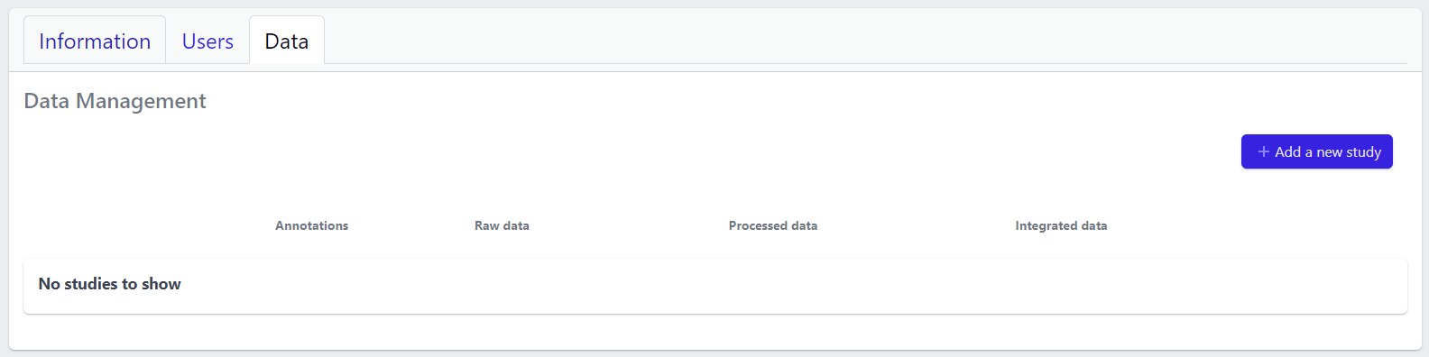
In the upper right corner an Add a new study button allows creation of new studies. Please see here for more details on how to add a new study to the project.
Existing projects
Once studies have been created, the page shows a list of studies:
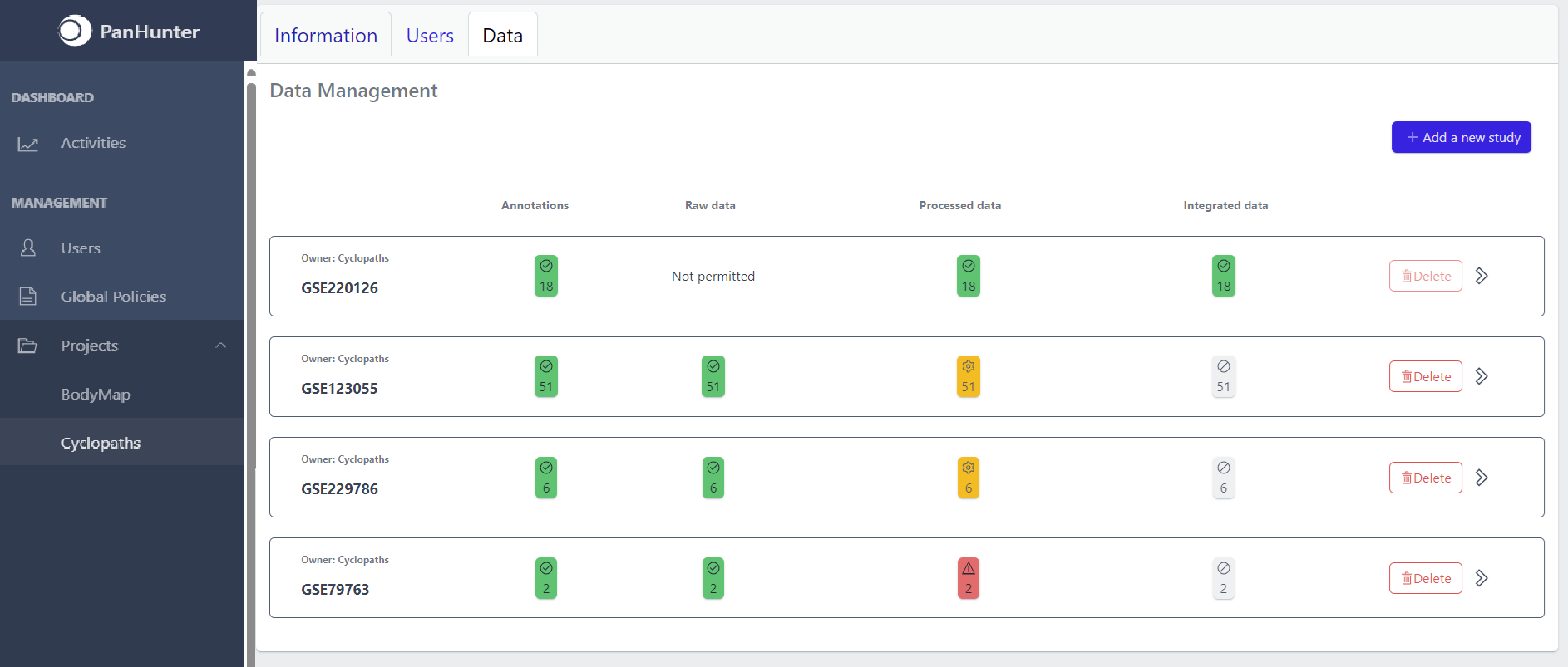
Each row corresponds to the single study, with a graphical visualization of data upload pipeline through the different stages of sample lifecycle:
- Annotations - Shows the number and the status of created (uploaded) samples that are annotated with metadata
- Raw data - Shows the number of samples with raw data and indicates the status of raw data stage
- Processed data - Shows the number of samples with processed data and indicates the status of processed data stage
- Integrated data - Shows the number of samples with integrated data and indicates the status of the integrated data stage
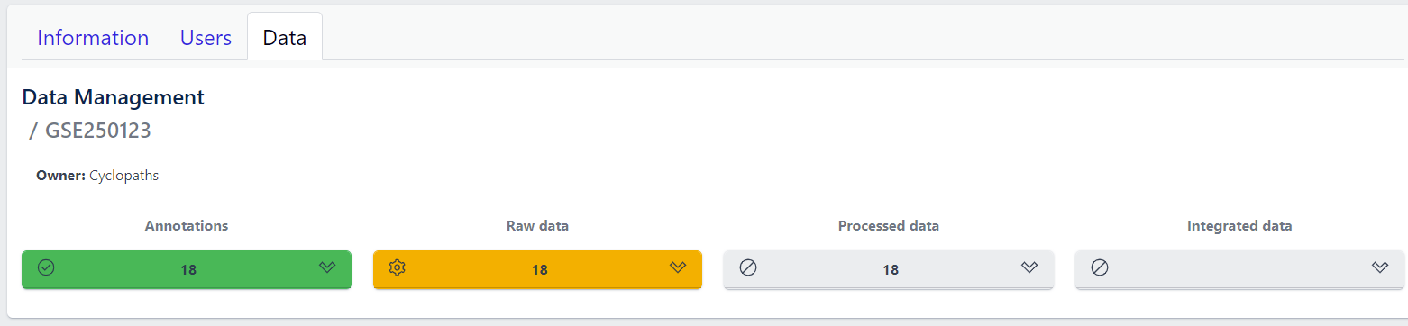
The colour of the tiles indicates the status for each data upload stage described above:
- Grey - data is not yet available for this stage
- Yellow - the stage is ready for upload, import, processing or integration of samples
- Blue - the process is running for this stage
- Green - the process has successfully finished for this stage and samples are correctly annotated, raw data is imported, processed or integrated
- Red - the process for this stage has failed
Detailed view of the study
Clicking on a study row leads to the detailed view of the study, which shows the same information as the overview page, but for a single study. Here, the tiles can be unfolded with a click, displaying more information about the current status of the specific data upload stage.
Additionally, the detailed view of the study enables user to perform operations like sample import, raw data inport, data processing and integration.
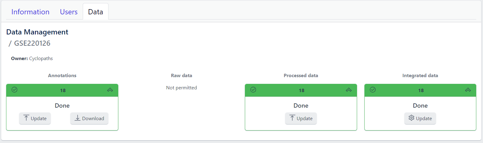
To navigate back to the overview page, click on the Data Management at the top left of the content area.
2.3 - Data upload
1. Creating new study
Step 1: New studies can be created in the project by clicking on the Add a new study button in the top right corner of the data overview page.
A pop-up window appears:
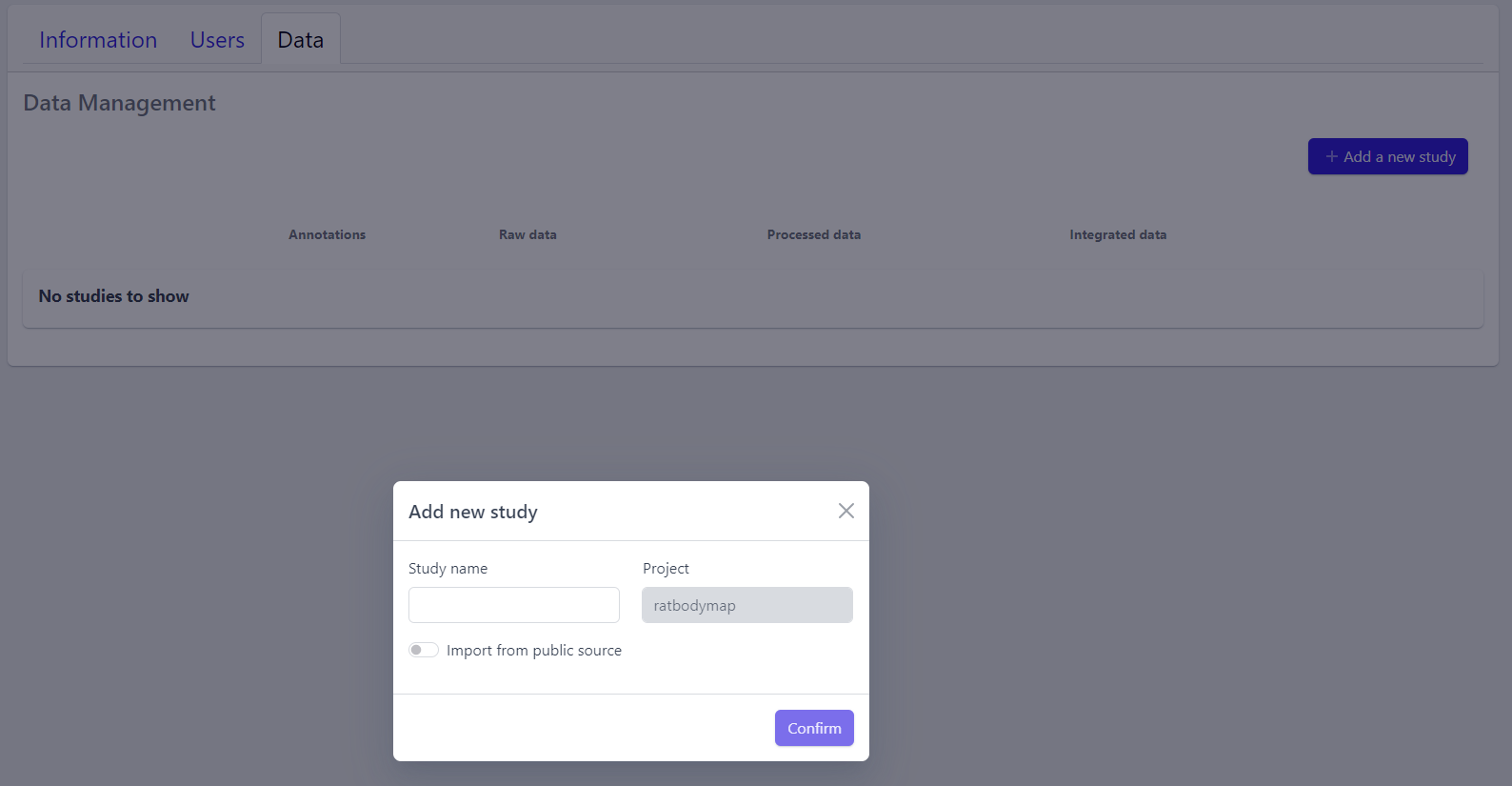
Based on the source the data is coming from, the process can be slightly different:
To upload proprietary data or other custom datasets, the process is as follows:
Step 2: Enter a study name in the pop-up window
Step 3: Click on Confirm
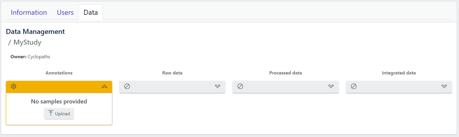
The new study will appear in the studies overview table as a new row, but without any associated samples. The Annotations tile will be coloured yellow with No samples provided status, indicating that the pipeline is ready for sample table upload.
However, with PanHunter it is also possible to import studies directly from public sources.
Direct import from public sources is at the moment supported for Gene Expression Omnibus (GEO), a genomics and transcriptomics database, that freely distributes high-throughput expression data submitted by the scientific community. Datasets are identified by so-called accession numbers (e.g. GSE22423).
Downloading GEO dataset directly from the database can be done with few additional steps:
Step 2: Activate Import from public source option
Step 3: Select GEO Datasets as a Public source
Step 4: Enter a valid GEO Accession number
Step 5: Click on Confirm
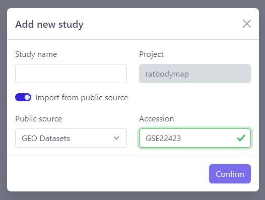
Panhunter will search for the given dataset accession number in GEO and download sample metadata. If successful, a pop-up window for sample table validation appears and user can proceed with Step 2. of sample table validation.
2. Sample table upload and validation
💡 More details about sample table file can be found under data formats supported.
Once study is successfully created, and Annotations tile is yellow with No samples provided status. This means that we need to upload samples, which is done via sample table upload and validation.
Step 1: To upload samples from a sample table Excel file, click on the Upload button on the Annotations tile and select a file from your computer to import.
📝 In case study is imported from public sources, this step is done automatically.
Step 2: Sample table validation
After the uploaded file is successfully read by PanHunter, a pop-up window to perform sample table validation appears, as displayed below:
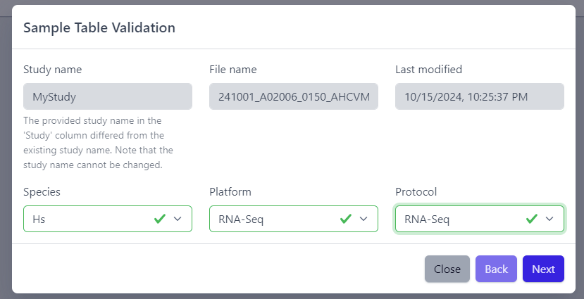
Please note that the Study name, File name and Last modified can not be edited directly. The Study name is defined during the creation of the study, and is taken from the Study column in the sample table file. File name and Last modified are defined by the file itself. To change the study name, please update the sample table file localy and restart the upload.
After you confirmed that Species, Platform and Protocol are correctly preselected, you can start the process of sample table validation by clicking on the Next button.
The result of sample table validation are shown in the same pop-up window:
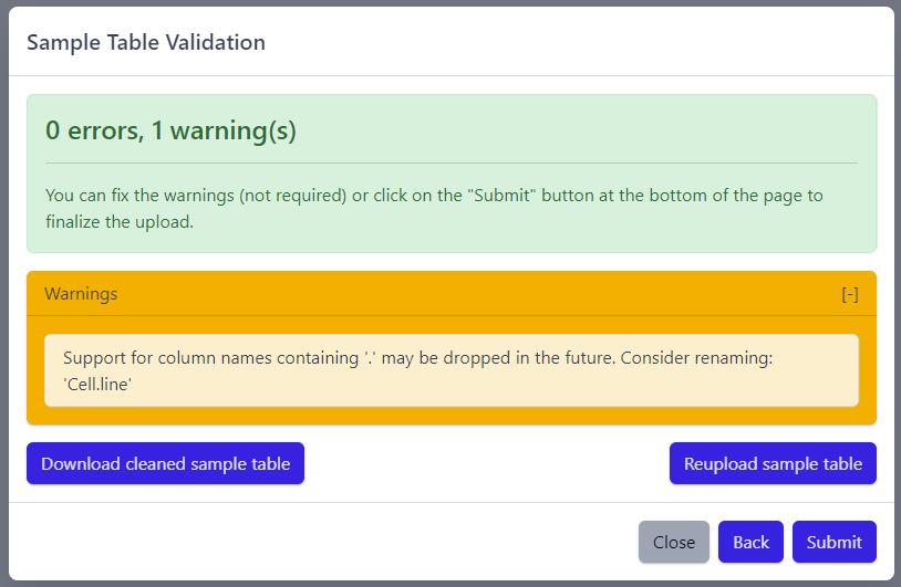
In case of errors (red), the sample table needs to be adapted. If this is the case, it is possible to use the Download cleaned sample table button to get the sample table file and modify it locally. Once sample table is modified as needed, click on the Reupload sample table button to upload the new version. The validation will be run again.
Please note that fixing warnings (yellow) is not required, but is recommended.
Step 3: Finish sample import
Once the validation passed without errors, click on the Submit button and samples will be imported and added to the study. Successfull upload of samples and study metadata will be indicated in the study details view as a green Annotations tile and the yellow Raw data tile, which indicates that the pipeline is ready for import of raw data.
3. Raw data import
After studies are successfully created and samples are uploaded, the yellow coloured Raw data tile indicates that the pipeline is ready for upload of raw data.
📝 Info: Import of raw data via the user interface is currently supported for GEO (link) and proteomics datasets. In case you have other types of data, please contact PanHunter Support.
Step 1: Expand yellow Raw data tab in the detailed study view
Step 2: Click on the Import button
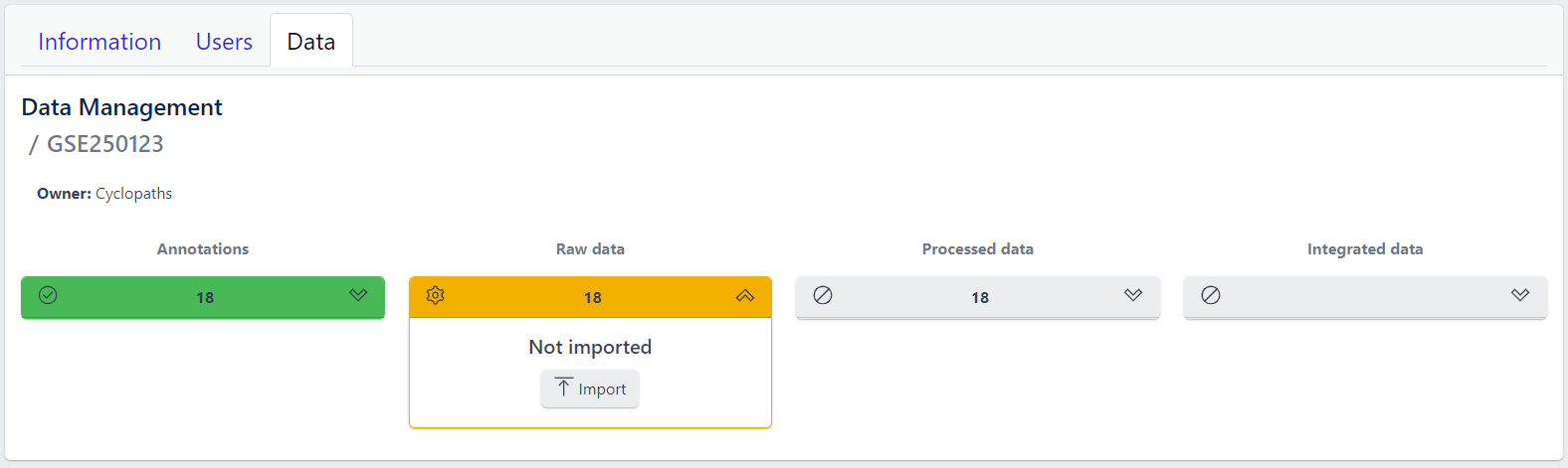
After starting the import, raw data files will be downloaded directly from GEO, with no additional input from user required.
To import output files of mass spectometry instruments, please fill in all required information in the pop up window and select files from local storage to be uploaded.
💡 This section is currently in progress - for more information please contact PanHunter Support.
Once import of raw data is initiated, a background job is started on the server. Blue coloured Raw data indicates that the process is running.
Once the import of raw data is sucessfully completed, Raw data stage is coloured green and displays the number of samples for which raw data is available. Additionally, Processed data tile is coloured yellow, indicating that the data is ready for processing.
In case an error occurs, it is indicated by the red Raw data tile that can be expanded via click to investigate the job output.
4. Data processing
Once raw data is available for imported samples, you can proceed with data processing. The data is ready for processing once Annotations and Raw data stages are successfully finished, and thus coloured green, and Processed data is coloured yellow with Not processed status.
Step 1: Unfold Processed data tile in the detailed study view.
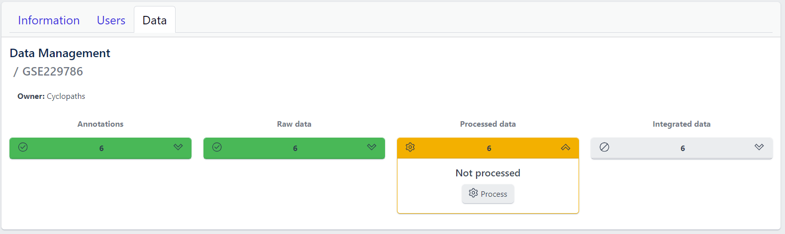
Step 2: Click on the Process button
Once the processing is initiated, a background job is started on the server. Blue coloured Processed data indicates that the job is running. Please keep in mind that depending on dataset sizes, these jobs may run for multiple hours or even days.
Once sucessfully completed, the Processed data stage turns green, displaying Processed status. Additionally, Integrated data tile is now coloured yellow, indicating that the data is ready for integration.
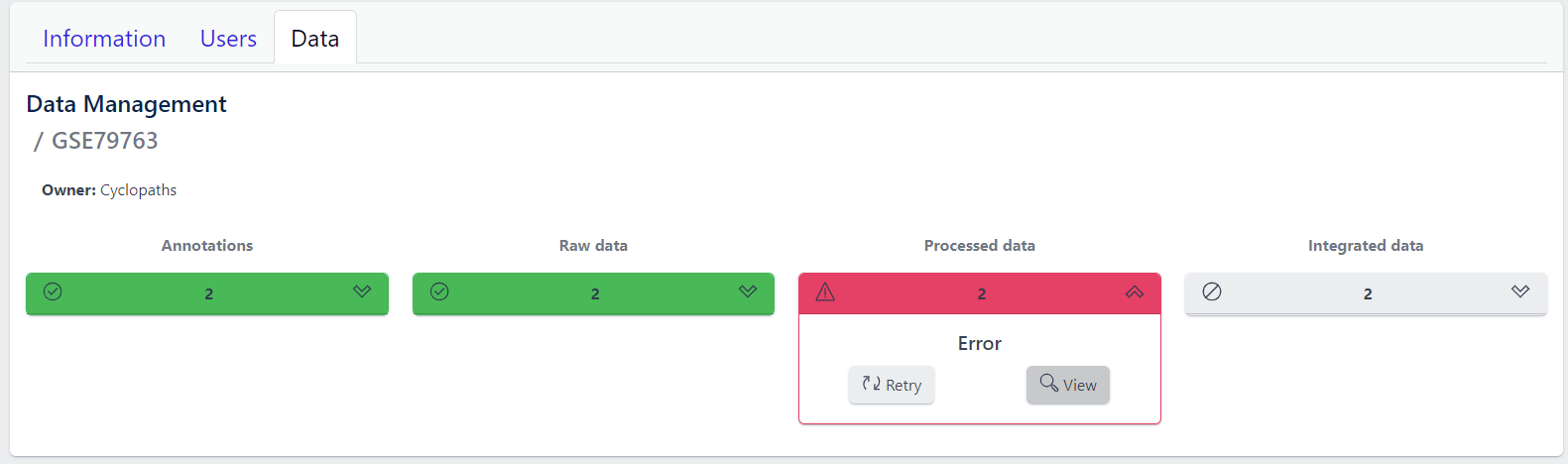
In case of a failure, Processed data stage turns red displaying Error status. To investigate what went wrong, please click on the View button to see output of the job. Clicking on the Retry button will start data processing again.
5. Integration of processed data
Once processed data is available in the study, the data is ready to be integrated to PanHunter. The pipeline is ready for integration once Processed data is coloured green and Integrated data is coloured yellow. Data will be available in PanHunter only after integration process is successfully finished.
Similar to the previous stages described above, the Integrated data tile in the study details view allows to run data integration jobs.
Step 1: Unfold Integrated data tile in the detailed study view.
Step 2: Click on the Integrate button
Clicking on the Integrate button starts a background job on the server. While the process is running, the Integrated data tile will be coloured blue.
Once sucessfully completed, the Integrated data stage turns green and data automatically becomes available in PanHunter apps.
In case of a failure, the Integrated data turns red displaying Error status. To investigate what went wrong, please click on the “View” button to see output of the job. Clicking on the Retry button will start data processing again.
2.4 - Updating data
Studies already created and existing in PanHunter, can be updated at any time via detailed study view. This can be done at any stage of data upload pipeline, regardless whether the study has been fully integrated into PanHunter or not.
Updating samples
In order to modify the sample metadata, to either correct or add additional information, it is possible to download and re-upload sample table files via the green Annotation tile in the detailed study view. This can also be done when the raw data have been added, processed and integrated already.
The process is similar to creating new samples as described in here, except that in this case it’s possible to start with sample table that is already available for the study.
- Download button downloads existing sample table which can then be modified locally
- Update button enables upload of updated, changed or newly created sample table. Please note that this will trigger sample table validation process again. Successful update of the sample table will overwrite existing sample table, update the sample information in the project and the additional or modified metadata will be available in PanHunter apps.
Notes
- Depending on the app, reload the of the app in the browser might be required in order to see the new information. In new information is not available after reload, please close the app and wait three minutes to make sure the app process on the server stopped. Opening the app again will force a reload of all data which includes the new information added.
- Samples will be available in PanHunter apps only when the value of the Status column in the sample table is set to Analyzed. This is usually done automatically when data has been processed and integrated. If sample information is modified, there is no need to change the status of samples unless changes have an impact on data processing and integration. In this case processing and data integration need to be re-run.
Updating data
In case update of data is required, this can be done for any stage at any time. To re-upload raw data or re-run processing and/or integration, please use Update button for respective data upload stage in the detailed study view.
Please note that updating raw or processed data requires re-integration of the data as well.
2.5 - Deleting studies
Delete a Study
Deleting a study from PanHunter is possible directly in the overview of available studies in Data tab via Delete button.
Clicking on the Delete button will trigger a pop-up window to confirm deletion of the study.
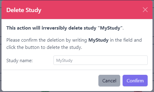
Please note that at the moment, possibility to delete study depends on the study data type (e.g. RNA seq data). In case you experience issues, please contact PanHunter Support.