From differential expression to pathway enrichment
This guide walks you through a complete analysis from raw samples to enriched pathways. You will:
- select the samples you want to compare,
- check how the samples group in a dimension reduction plot,
- calculate a differential expression (DE) comparison,
- inspect the differentially expressed genes,
- run an over-representation analysis (ORA) on pathways and
- look at a single pathway with the expression changes mapped onto it.
The guide takes about 20 minutes, most of it waiting for the calculation to finish.
Before you start
- Access: You need access to a PanHunter project and permission to calculate comparisons in it. If the Comparison Calculation tab is missing or the submit button stays disabled, ask your project leader.
- Example data: The guide uses the study Yu2014, a public rat body map (GSE53960) with eleven tissues from rats of different ages and both sexes. As an example question we compare liver samples from old rats (104 weeks) with liver samples from young rats (6 weeks). If your project does not contain Yu2014, follow the same steps with your own study and replace tissue, factor and levels accordingly.
- Background: If you are new to DE analysis or enrichment analysis, the pages Differential gene expression analysis and Enrichment analysis explain the methods behind the steps below.
Step 1: Select the samples
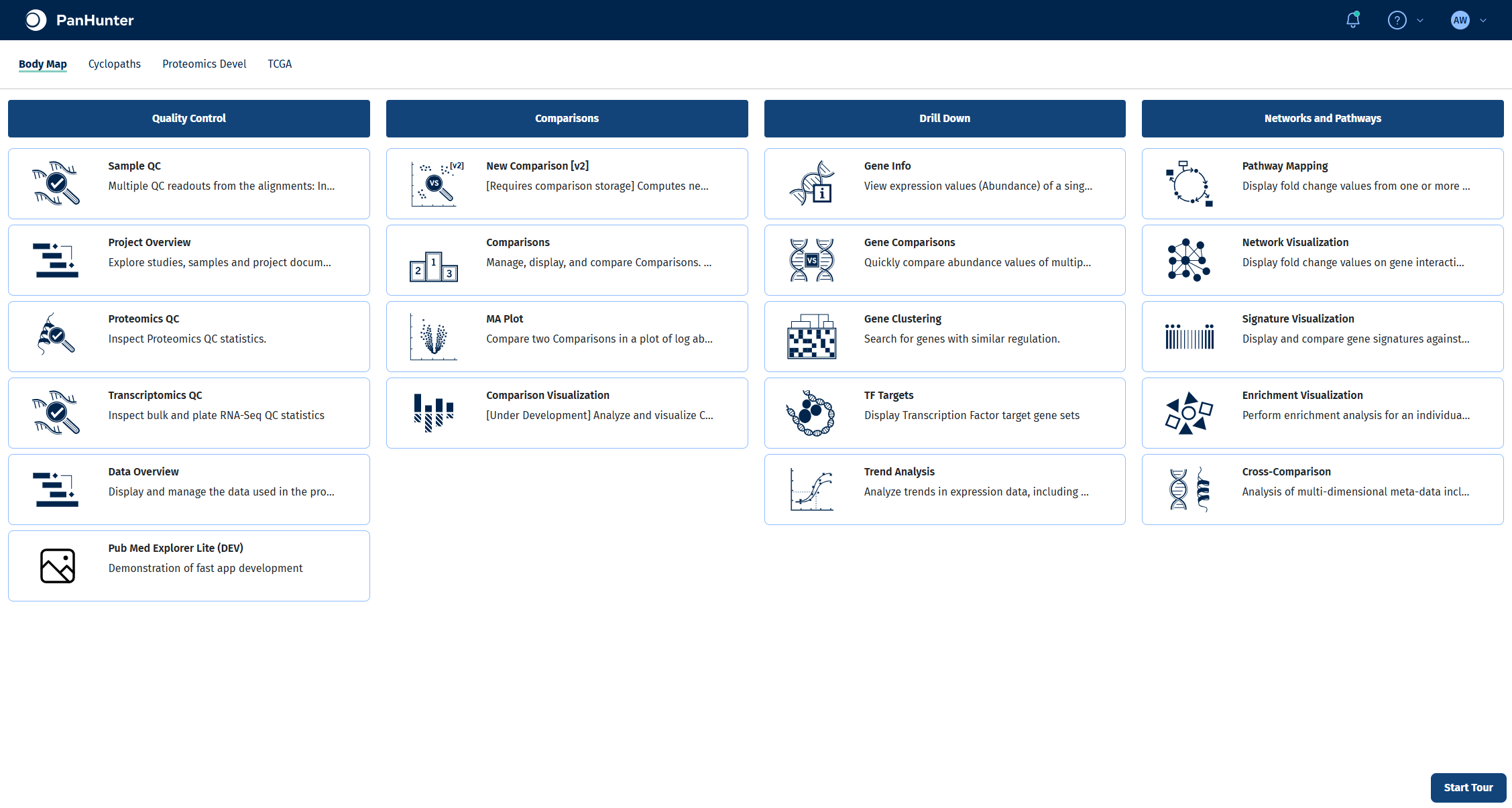
All steps up to the calculation happen in the New Comparison [v2] app. Open it from the start page of your project.
Selecting samples in the Sample Selector panel on the left defines which samples every tab of the app works with, including the comparison you calculate later. Narrowing the selection down to exactly the samples of your question keeps plots readable and makes sure the statistical model is only fitted on relevant samples.
- In Studies, select Yu2014. The panel shows how many samples were loaded.
- In Add a new modifier, choose Filter categ. and click +.
- In the new filter, set Filter to Tissue, keep Include and select Liver in Values.
- Add a second Filter categ. modifier with Filter set to Age and Values set to 6 and 104.
For more on modifiers, see the Sample Selector documentation.
Check your result
The Sample Selector panel reads Loaded 15 out of 316 samples and shows the two filters Tissue: Liver and Age: 6, 104.
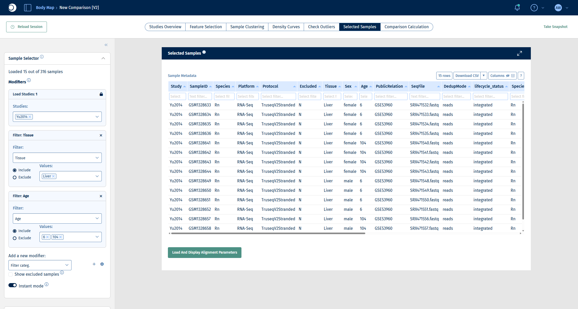
Note: The Studies Overview tab summarizes the whole study and does not reflect the filters. Use the Selected Samples tab to see the samples that are actually selected.
Step 2: Explore how the samples group
Before calculating a comparison, checking how the samples relate to each other tells you which factors drive the biggest differences in your data. Factors with a visible effect that are not the subject of your question are candidates for the comparison formula, so that the model can account for them.
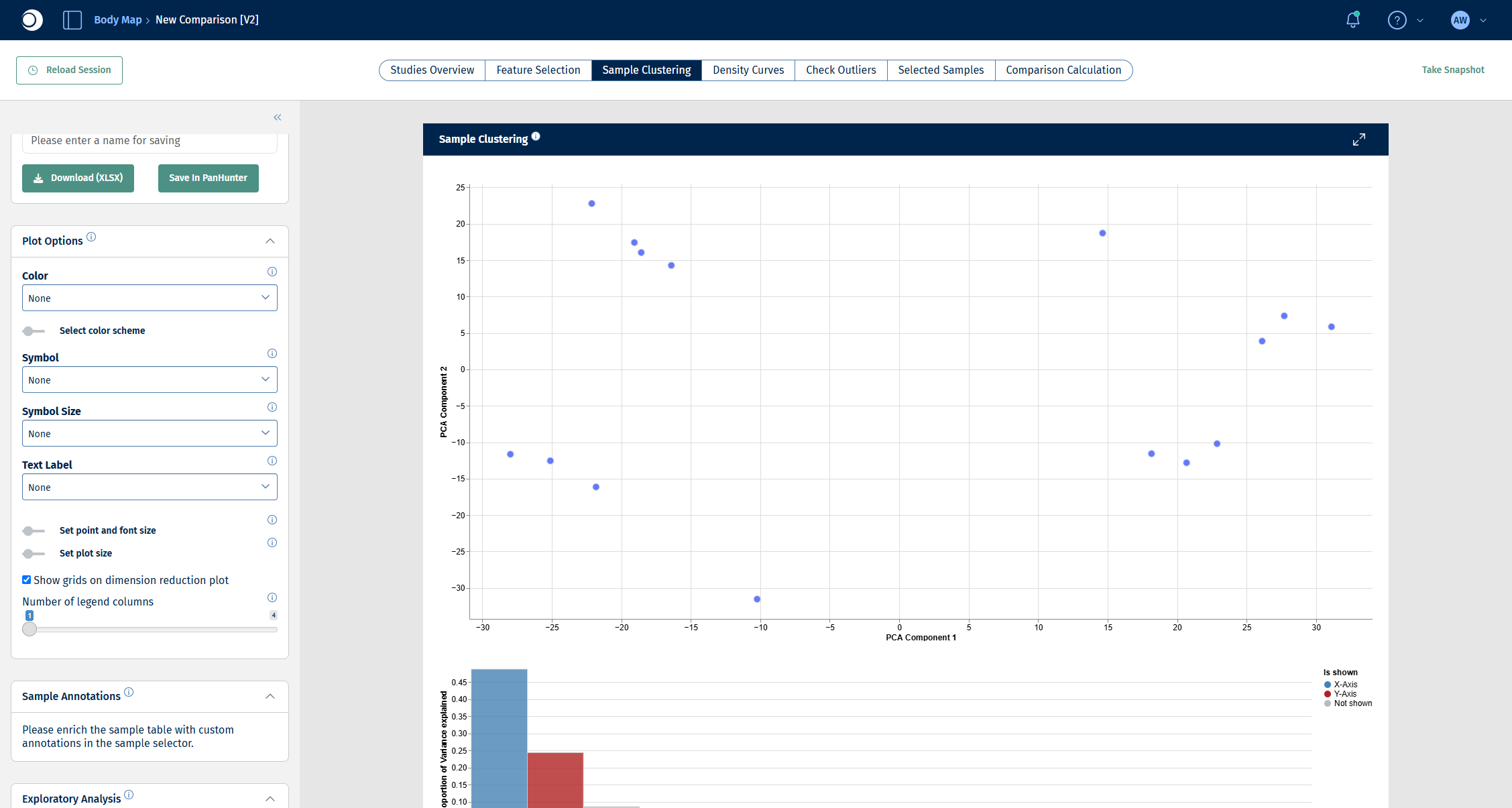
- Open the Sample Clustering tab. It shows a PCA of the selected samples.
- In the left sidebar, scroll down to Plot Options.
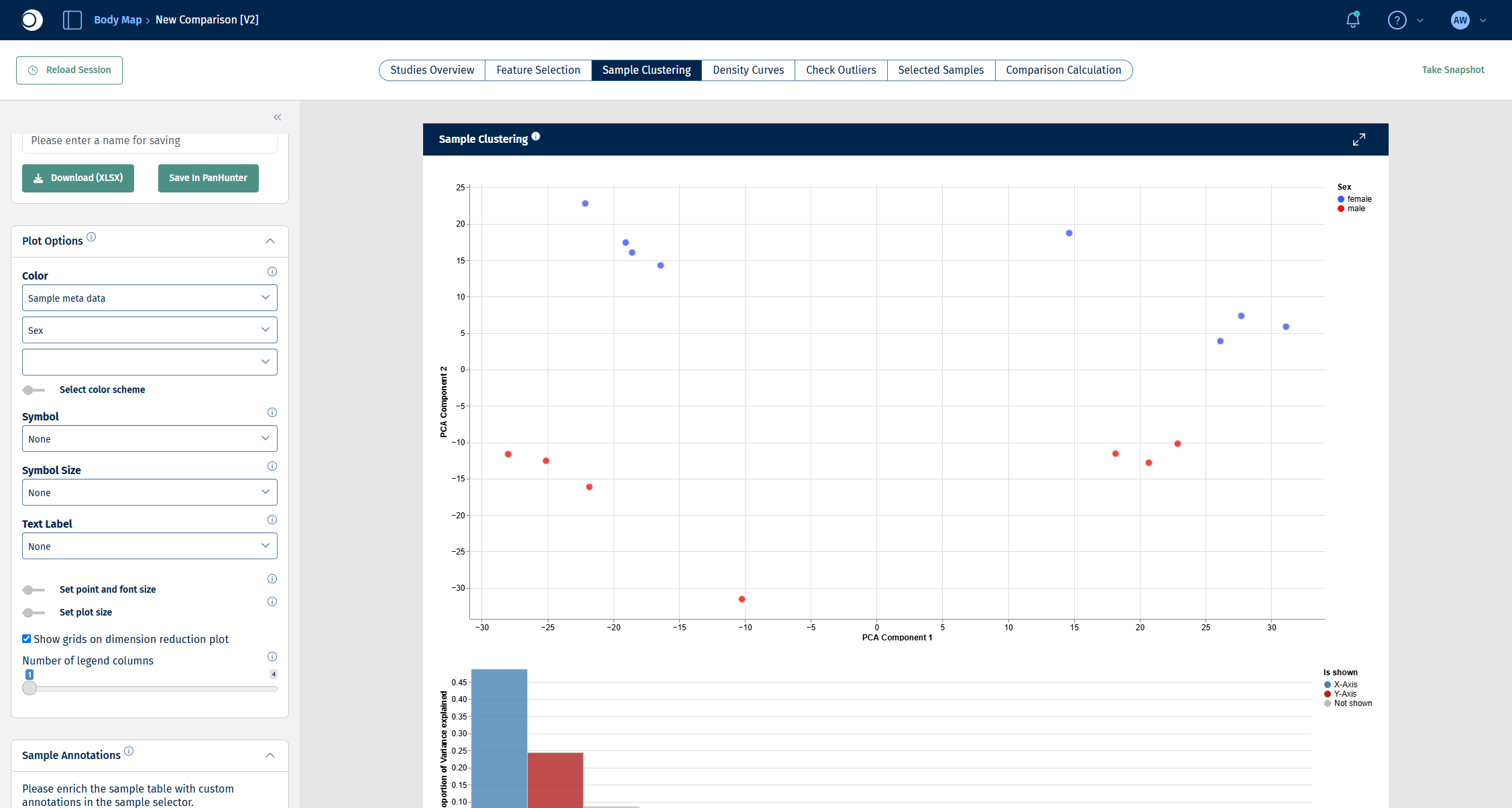
- Set Color to Sample meta data and pick a metadata column, for example Sex.
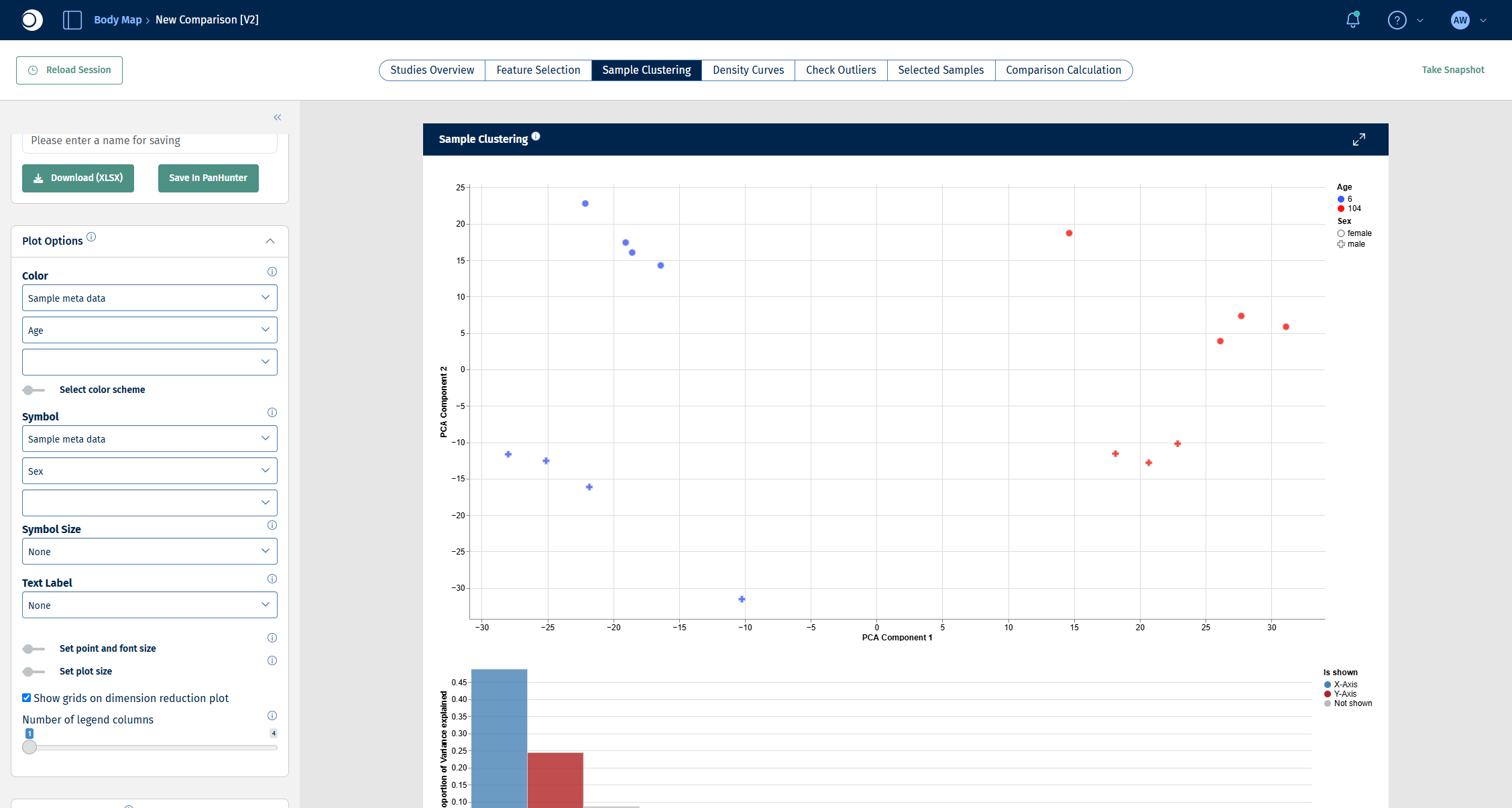
- Switch the color column to Age and set Symbol to Sample meta data and Sex.
Try other columns as well: coloring by different metadata is the quickest way to spot batch effects or unexpected groupings. For all options, see Plot Options panel and Dimension Reduction panel.
Check your result: PCA without coloring
Check your result: PCA colored by sex
The samples split along the second principal component (y-axis) by sex.
Check your result: PCA colored by age, symbols by sex
The samples split along the first principal component (x-axis) by age: 6-week samples on the left, 104-week samples on the right. Age explains the largest part of the variance, sex the second largest. That is why the comparison in the next step includes both factors.
Step 3: Set up and validate the comparison
The Comparison Calculation tab defines which groups are compared and how. A single run can create many comparisons at once; for this guide one comparison is enough. All fields are described in detail in New Comparison: Comparison Calculation.
- Open the Comparison Calculation tab.
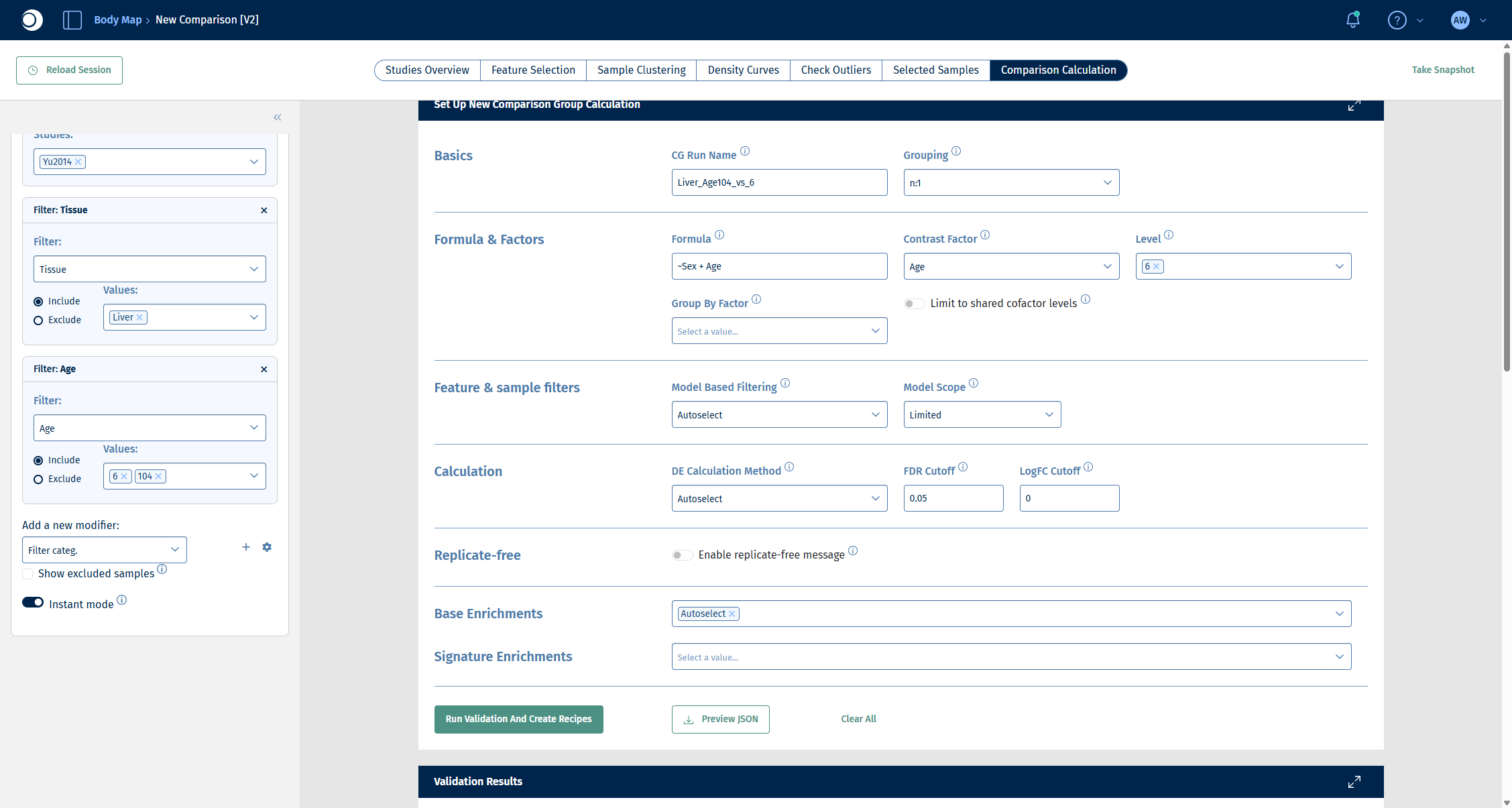
- Under Basics, enter a CG Run Name, for example
Liver_Age104_vs_6, and keep Grouping at n:1. The name must be unique in the project; in the screenshots of the later steps the run is calledGuide_Liver_Age104_vs_6. - Under Formula & Factors:
- enter the Formula
~Sex + Age. Including Sex lets the model account for the sex difference you saw in step 2, so that the comparison isolates the effect of age. - set Contrast Factor to Age.
- set Level to 6. The level you select here is the reference (denominator); the remaining level, 104, becomes the numerator.
- enter the Formula
- Leave Feature & sample filters, Calculation and Base Enrichments at their defaults (Autoselect).
- Click Run Validation And Create Recipes.
Important: Factor names in the formula are case-sensitive and must match the metadata column names exactly.
Check your result: set-up
Validation checks your set-up without calculating anything. The Validation Results section lists errors, warnings and info messages, followed by the comparisons (recipes) that would be calculated.
Check your result: validation
- Errors (0) and Warnings (0).
- Info (3): default enrichment analysis with wikipathways (fisher), gobp, gocc and gomf (weight); DE method autoselected as deseq2 based on the number of samples; no model-based filtering.
- Created recipes (1): one recipe 104-6 with 7 numerator and 8 denominator samples.
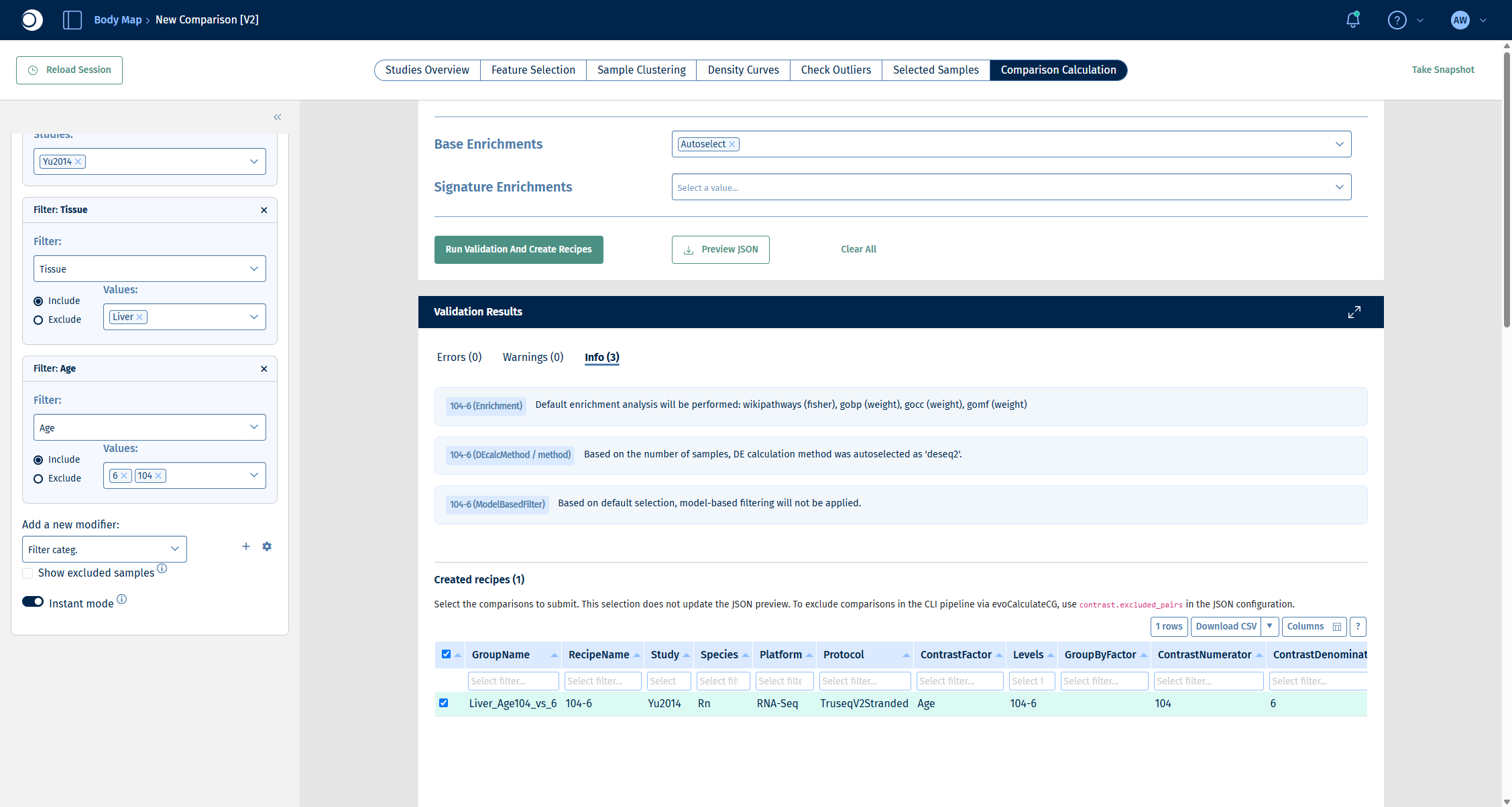
The wikipathways (fisher) enrichment in the info messages is a pathway over-representation analysis that is calculated together with the comparison. You will explore enrichments interactively in step 5.
Step 4: Run the calculation and inspect the DE results
- Scroll down to the recipe table, make sure the recipe is checked and click Submit Calculation To SLURM.
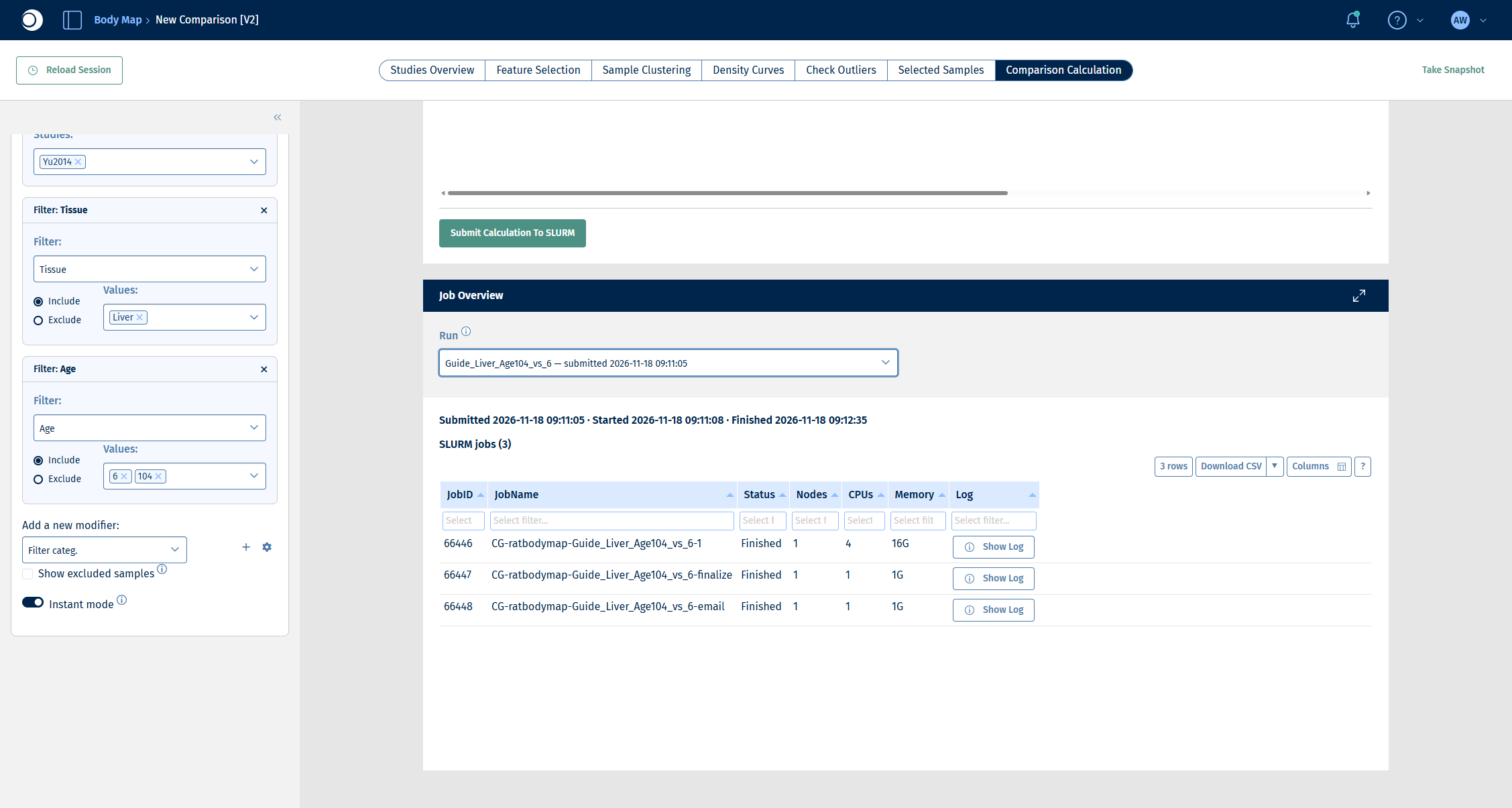
- Follow the progress in the Job Overview section. Select your run in Run. A run consists of three jobs: the calculation itself, a finalize job and an email job. For this example the whole run takes about two minutes.
Check your result: job overview
All three jobs show the status Finished.
When the run has finished, open the Comparisons app from the start page.
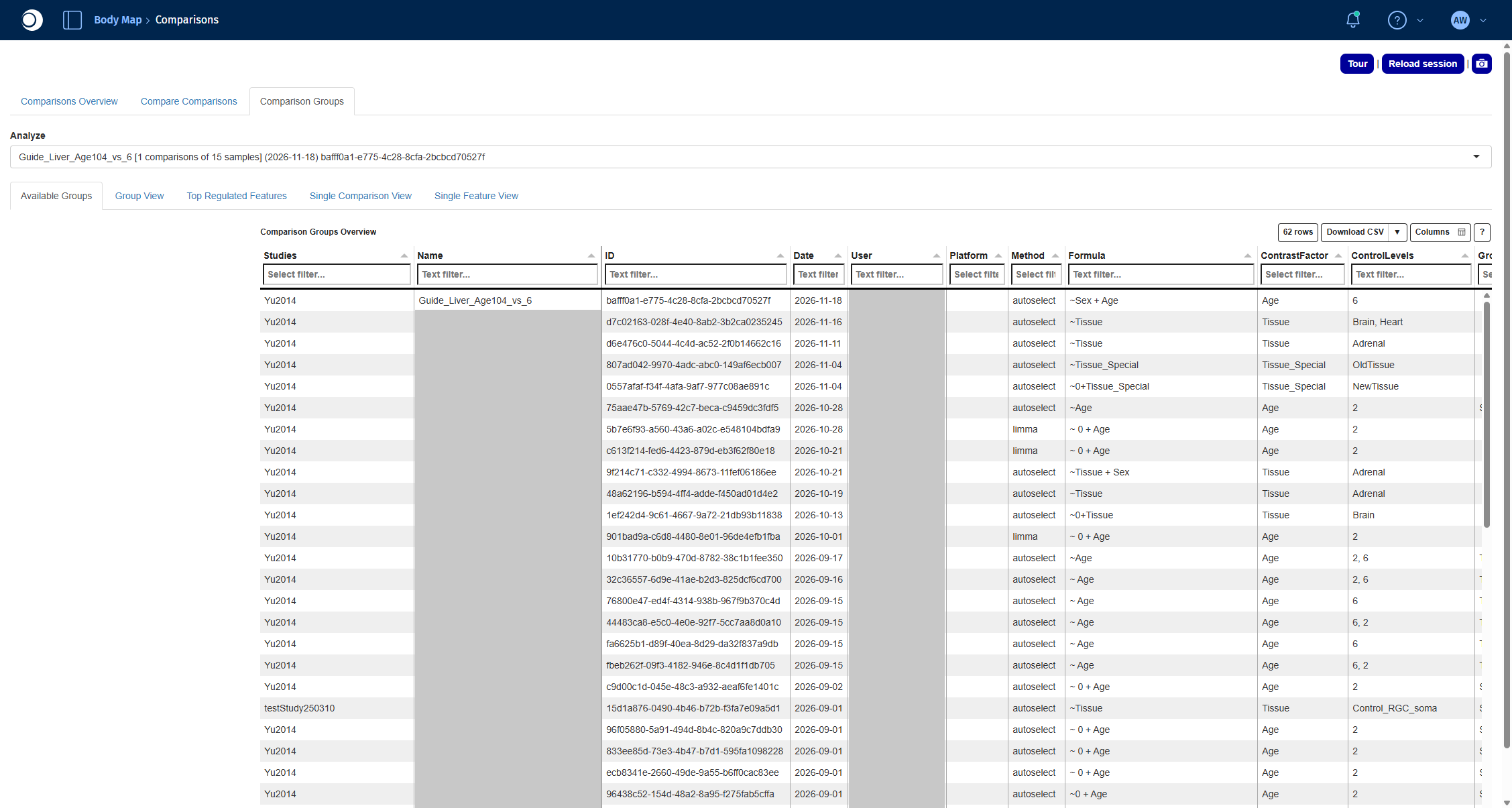
- Open the Comparison Groups tab. Comparisons calculated in the Comparison Calculation tab are listed here, grouped by run. In Analyze, select your run.
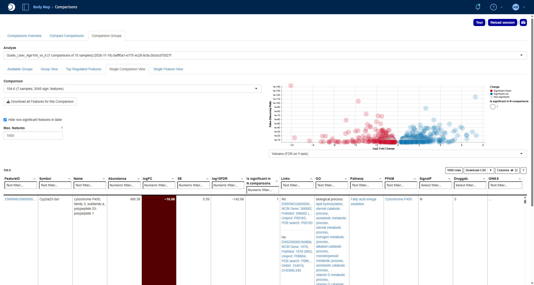
- Open the Single Comparison View tab and select the comparison 104-6 in Comparison.
The volcano plot shows the fold change (x-axis) against the significance (y-axis) of every gene; red genes are significantly down, blue genes significantly up in old compared to young liver. The table below lists the significant genes with their fold change, FDR and links to external databases. For all functions of the app, see Comparisons.
Check your result: Comparison Groups
Check your result: DE results
The comparison reads 104-6 (7 samples; 3545 sign. features). The most strongly changed gene is Cyp3a23/3a1, a cytochrome P450 enzyme, with a log2 fold change of about −10.
Step 5: Find over-represented pathways
An over-representation analysis tests whether the differentially expressed genes contain more members of a pathway than expected by chance. The Enrichment Visualization app runs this test for any gene set collection and shows the results as plots and tables.
- Open the Enrichment Visualization app from the start page.
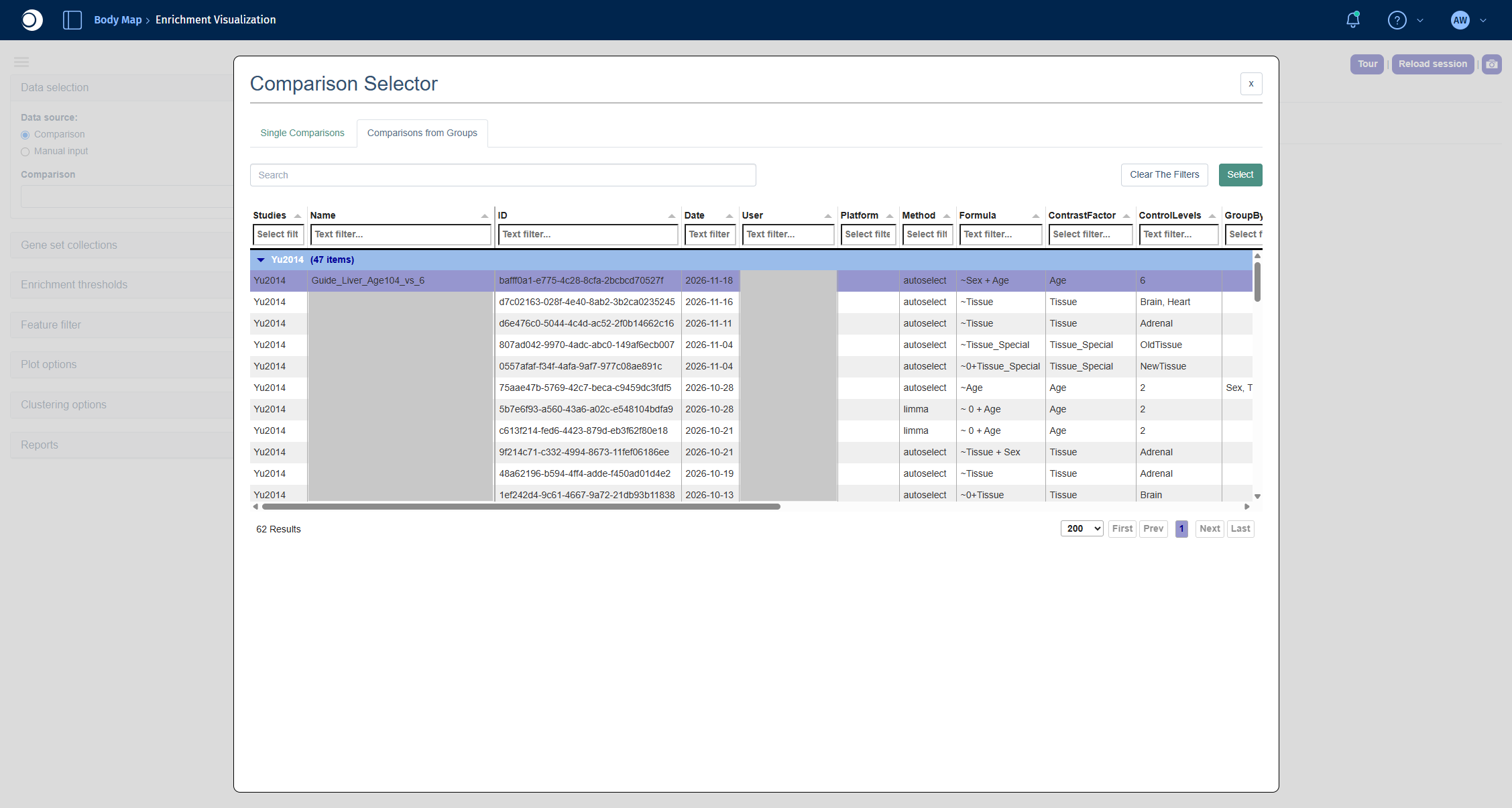
- Under Data selection, keep Comparison as data source and click into the Comparison field. The Comparison Selector opens.
- Open the Comparisons from Groups tab, select your run and click Select. In the next view, select the comparison 104-6 and click Select again.
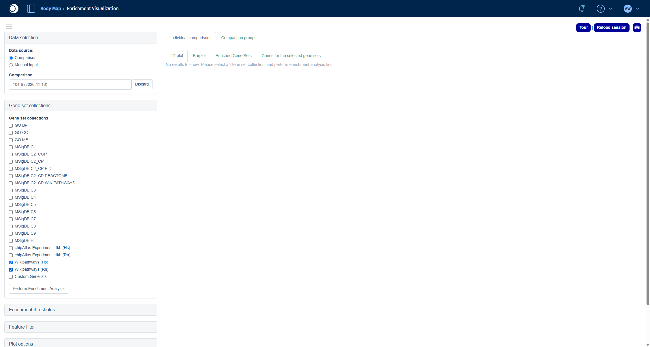
- Open Gene set collections and check Wikipathways (Hs) and Wikipathways (Rn).
- Click Perform Enrichment Analysis.
Recommendation: For non-human data, always add the human collection (here Wikipathways (Hs)) to the collection of your species. Human pathways are annotated much more comprehensively, and PanHunter maps your genes to their human orthologs. In this example, Wikipathways (Rn) alone finds only two enriched pathways, together with Wikipathways (Hs) it finds 64.
Check your result: Comparison Selector
Check your result: gene set collections
The results are spread over four tabs:
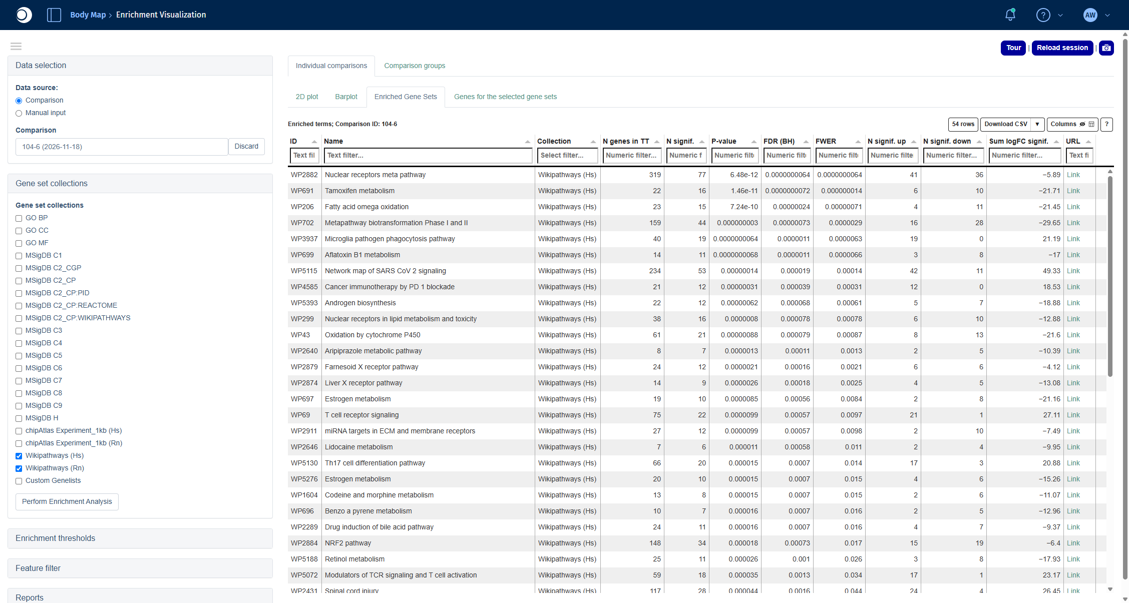
- Enriched Gene Sets: the table of enriched pathways with the number of genes, the number of significant genes up and down, p-value and FDR.
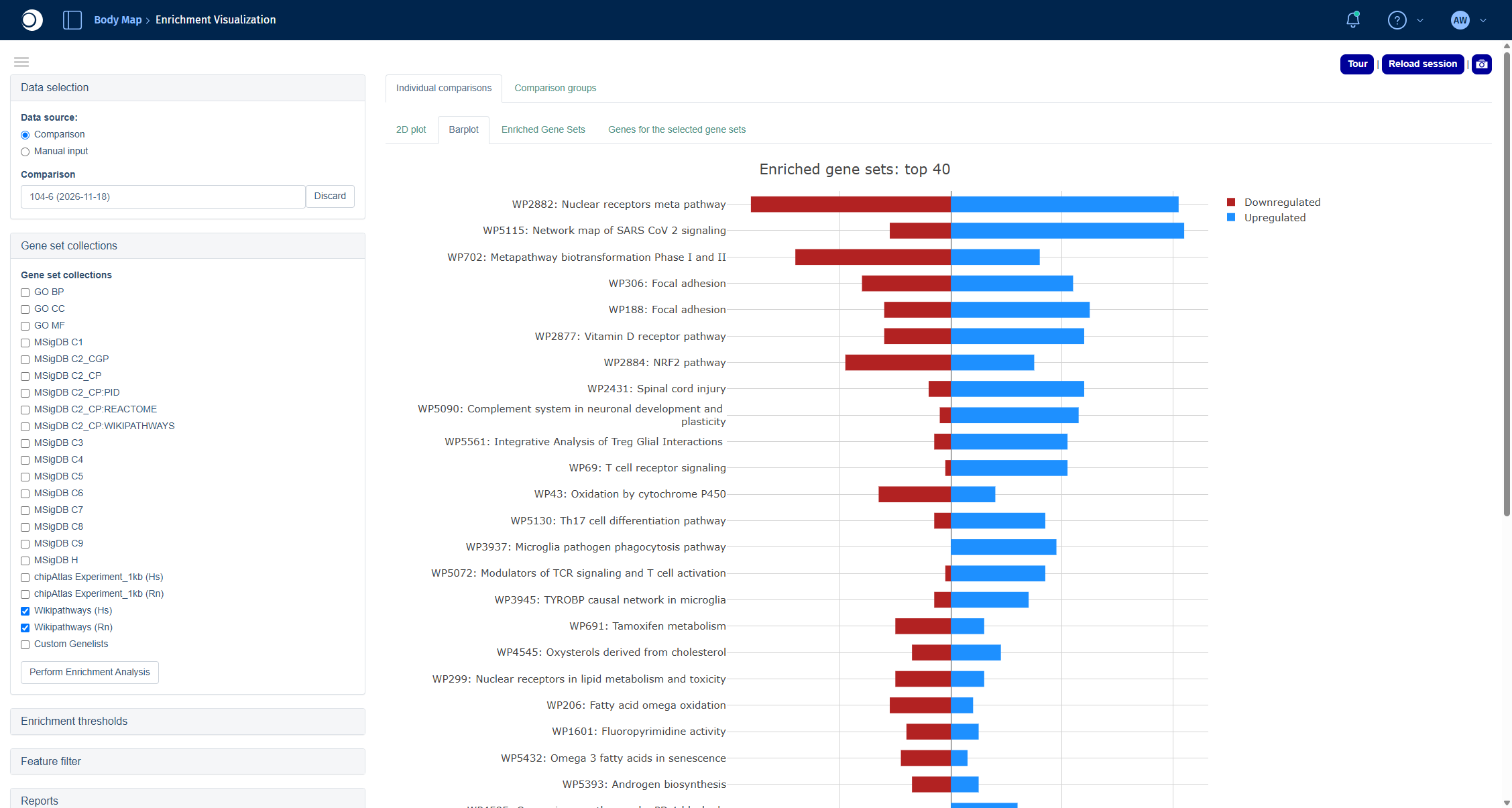
- Barplot: the top 40 pathways with the number of up- and downregulated genes.
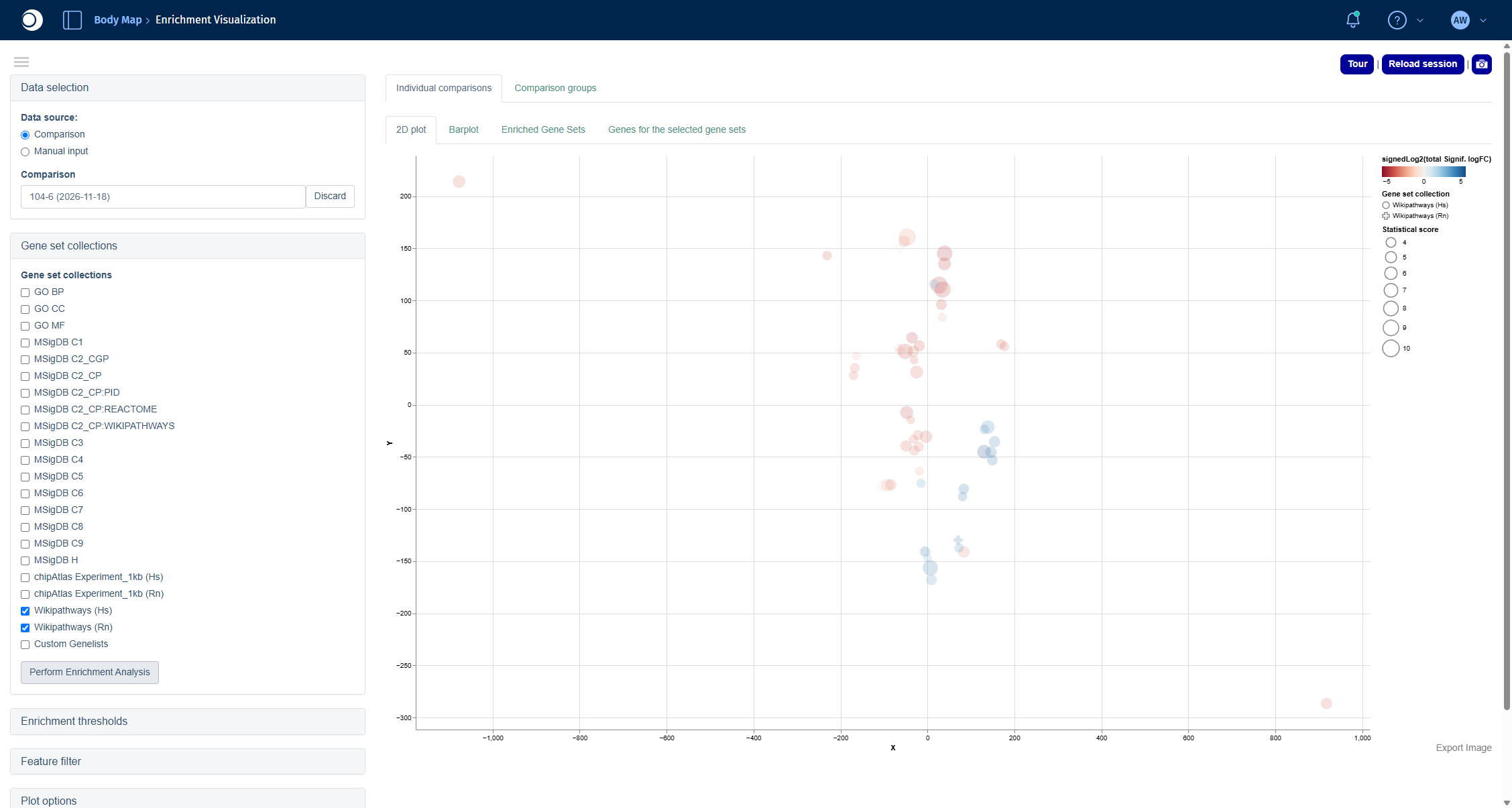
- 2D plot: pathways arranged by similarity of their gene content.
- Genes for the selected gene sets: the genes of the pathways you select in one of the other tabs.
For all options, including thresholds and filters, see Enrichment Visualization.
Check your result: enriched pathways
The table contains 64 pathways. Among the top hits are Nuclear receptors meta pathway, Tamoxifen metabolism, Fatty acid omega oxidation and Metapathway biotransformation Phase I and II, which points to changes in the drug and lipid metabolism of the aging liver.
Check your result: 2D plot
Each circle is an enriched pathway. Pathways that share many genes lie close to each other; the color shows whether the significant genes of a pathway are mostly down (red) or up (blue), the size shows the statistical score.
Check your result: barplot
Step 6: Look at a single pathway
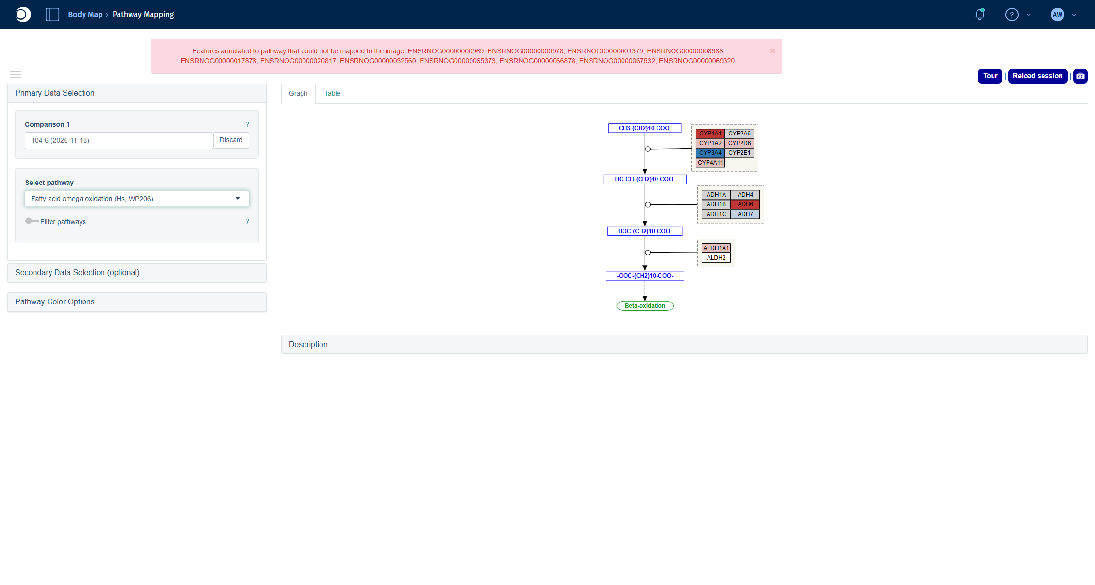
The Pathway Mapping app draws a pathway and colors each gene by its fold change, so you can see which parts of the pathway change and in which direction.
- Open the Pathway Mapping app from the start page.
- Click into Comparison 1 and select your comparison in the Comparison Selector the same way as in step 5.
- In Select pathway, type part of the pathway name, for example
omega oxidation, and select Fatty acid omega oxidation (Hs, WP206).
For coloring options and the table view, see Pathway Visualization.
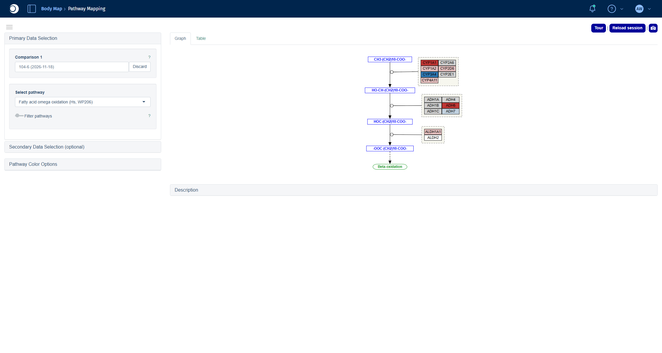
Check your result: pathway
The pathway shows the conversion of fatty acids along with the enzymes catalyzing each step. Red boxes are downregulated, blue boxes upregulated genes in old compared to young liver.
Troubleshooting
My new comparison does not show up in the Comparisons app.
Comparisons calculated in the Comparison Calculation tab are listed in the Comparison Groups tab, not in Comparisons Overview. In apps with a Comparison Selector, use the Comparisons from Groups tab. Make sure the run is finished in the Job Overview.
Pathway Mapping shows a red message about features that could not be mapped to the image.
The pathway contains genes of your comparison that have no counterpart in the pathway drawing, for example because the drawing is based on human genes. The message lists their IDs. The pathway is still drawn correctly for all mapped genes.
The Enrichment Visualization shows the message Assigning random coordinates.
The 2D plot needs a minimum number of enriched gene sets. If fewer pass the thresholds, the pathways are placed randomly. Add more collections (see the recommendation in step 5) or relax the Enrichment thresholds.
Next steps
- Compare your comparison with other comparisons in Compare Comparisons.
- Look at the genes of an enriched pathway in their interaction network with Network Visualization.
- Check which transcription factors could explain the expression changes with TF Targets.