Quality Control for Bulk RNA-Seq data

• 1: Starting quality control
• 2: Deeper look into SampleQC
• 3: QC clustering
• 4: Finalizing the Quality Control

1 - Starting quality control

General assesement in the Project Overview

In the project overview app, you can check the general parameters for your study, such as the sample size or if the important variables are visible in the details tab.

Investigating Alignment statistics

For further statistics about the data integration we need to go into the ‘Sample QC’ app. First, we are presented with the Alignment statistics tab, showing different histograms for quality parameters.

Number of input reads

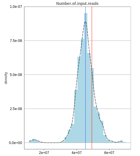
The first histogram is concerned with the number of input reads. While the blue vertical bar shows the median, the red bar shows the position of the current sample selected. A low number of reads can correspond to problematic data, while the definition of “low number” is sometimes subjective and numbers might depend on tissue type or species. Panhunter uses different color codes ranging from white to green to show low to high number of reads in the table below.

While absolute reads may be hard to distinguish by, big jumps should be investigated closely. While most of the data in the picture has 30-60 million reads, there are samples that have half or even less of the input reads. Taking these samples out should yield more homogeneous data which are more meaningful for further analysis.

Unique mapping

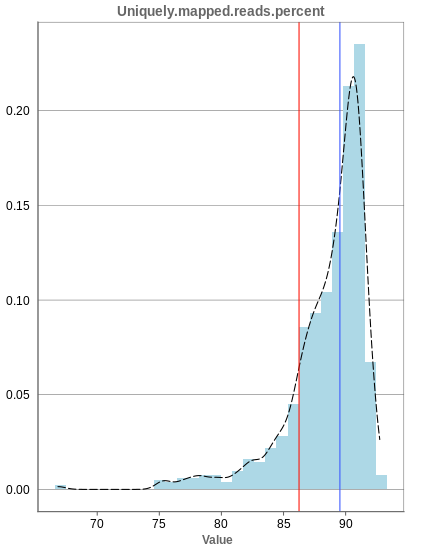
The general plot structure is similar to that of the number of input reads, such that we still want to detect outliers in the histogram. Because non-unique mappings of the input reads are not considered as reads in Panhunter, having a high percentage of uniquely mapped reads is very important.

While the displayed percentage above 85% is good for most samples, there is one with under 70% that should be omitted from the data. This also depends on the type of tissue that was used, such that the given number of 85% is considered meaningful for blood, but when using muscle cells, there might be much more lower numbers.

Mapping to multiple locations

While some reads are uniquely mapped, there is also the case of reads that are not mapped at all and reads that are mapped to multiple locations. As said before, these are not considered in the preprocessing of Panhunter, and only uniquely mapped reads are relevant for the count matrices.

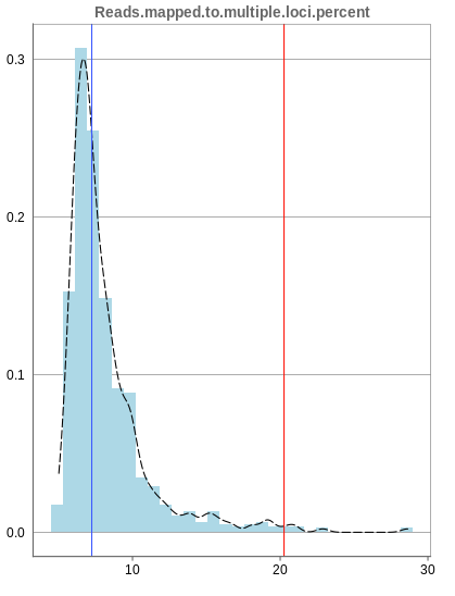
The remaining percentage of reads should largely be composed of multiple mapped reads, i.e. the number of reads that map to no location should be small.

2 - Deeper look into SampleQC

There are various other tabs in SampleQC, that are relevant for BulkRNA data.

Read distribution

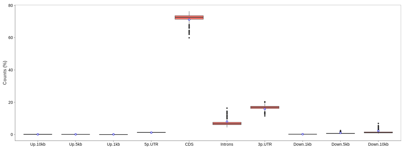
First of all, the box for total percentages should be ticked in the bottom for better comparison.

Ideally, the percentage of counts mapping to the highest should be CDS which stands for coding DNA sequence, relating to the region that codes for protein.

Also important is that up- and downstream are not mapped often.

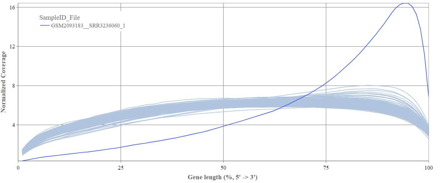
Gene body coverage

We can see the normalized coverage. The samples gene body coverages should be close to one another and should form a homogeneous band and, in BulkRNA-Seq, should be spanning quite ‘uniform’ over the gene length going down at the start and endpoints. Please note that evoenthouth this QC section is called gene body coverage we effectively measure the coverage along the RNA transcripts corresponding to the gene.

The sample colored in blue shows very untypical behaviour and is advised to be excluded.

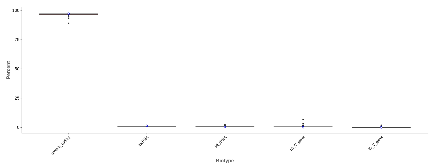
Biotype

The biotype (that is functional types of the genes to which reads are mapped) can be used for quality control. The protein_coding should be the highest and not far away from 100%. We can also see in our example that there we have IgC and IGv genes for tuberculosis data, which seems reasonable because they are relevant for the immune/antibody system of humans.

Mitochondrial

Usually, the proportion of transcripts mapping to mitochondrial genes should be low. If there is phenomenons such as cell death, the amount of mitochondrial transcripts increases and we might infer a lower quality for the data.

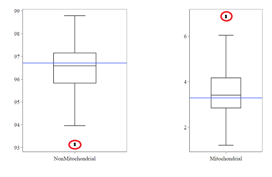
In our example, it may be useful to take out the two circled samples because they are clear outliers from the rest of the data.

Genes

An additional evaluation can be done by looking into the Genes tab, checking which genes are counted the most. The interpretation of this analysis is experiment specific and requires knowledge of the biological system that is investigated.

3 - QC clustering

The quality of the data can also be inferred from gene expression profiles represented via dimension reduction methods. Suitable methods in Panhunter are PCA, t-SNE and UMAP. The ‘New Comparisons’ app should be used in the following.

Clustering by sex

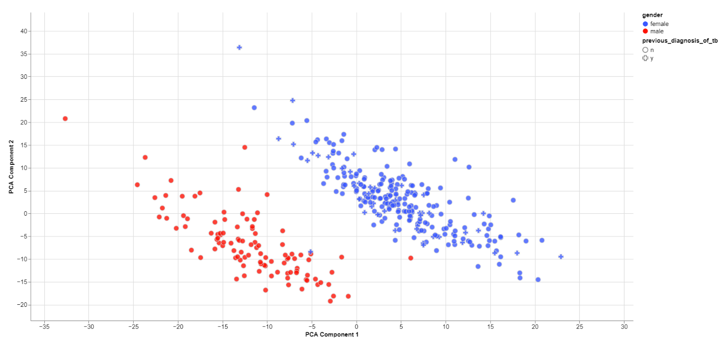
The biological sex should always be one of the greatest disparities between data points because an entire chromosome is different. Thus, there may be reason to exclude samples that are truly different from the rest of their group. However, some studies list gender which should not be confused with the biological sex.

What can also be inferred from the plot is that, in this data set, only females have been diagonsed with tuberculosis before, leading to a dependence between gender and previous_diagnosis_of_tb. These relationships are very important because correlation explained by the previous diagnosis can in some cases be completely explained by the gender/sex association.

PCA features

The categorical and numerical variables that are responsible for the variance in the data can be calculated with the buttons shown below in the picture.

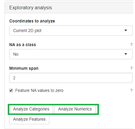
⚠️ Keep in mind that the default is to analyze only the current 2D plot of the dimensional reduction and may vary even by method (PCA,t-SNE, UMAP).

Check outliers

Even when there is no gender/sex variable present, there might be clear clustering. When comparing two groups, one can use the check outliers tab after selecting the groups, to look at up and downregulated genes and infer information from the results.

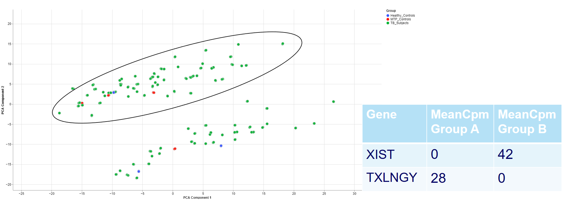
For example, the two groups are clustering completely different in the PCA plot. Even when there is no labeling variable, the comparison shows that certain genes are more present in the groups. Because the presented genes belong to the inactive X chromosome and the Y chromosome, we can infer that there are males and females in the data. This is important for quality control because of the large influence of the biological sex which might otherwise be neglected.

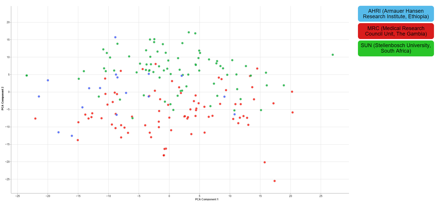
Clustering of other features

For one of the studies, different sites were used to collect blood samples from participants. This inevitable lead to differences that have to be accounted for and are thus important for the quality of the data.

4 - Finalizing the Quality Control

There are still various things that can be done to investigate the quality of the data but just a few final thoughts are mentioned down below.

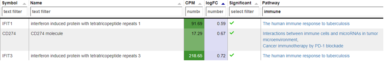
New comparisons

As outlook, one can fit a group comparison in the app ‘New comparisons’, tab ‘New comparison’ with relevant groups, such as TB_subjects against control. If important genes are up/downregulated, then this is another sanity check that can be done.

Reporting on the quality

If there are multiple studies, one could present as follows:

• general setup of the study, things that are noticeable immediately (samples missing)
• general QC stats
• clustering
• variables that are relevant and should be/should not be
• New comparison between important groups, i.e. treatment vs control
• short summary of the study, the QC and important conclusions
• general setup of the next study
• comparison of all studies
• Slide with table: study | sample | reason to take out