Guides
Step-by-step guides that walk you through a complete analysis across several PanHunter apps.
The pages in the PanHunter Apps section explain what each app does. The guides in this section start from a question instead: they take you through all apps you need to answer it, in the order you use them.
Each guide uses a public example dataset, so you can follow along step by step. At every important step, a collapsible Check your result box shows what your screen should look like. Try the step yourself first, then open the box and compare.
Available guides
1 - From differential expression to pathway enrichment
Compare two groups of samples, inspect the differentially expressed genes and find the pathways they are over-represented in.
This guide walks you through a complete analysis from raw samples to enriched pathways. You will:
- select the samples you want to compare,
- check how the samples group in a dimension reduction plot,
- calculate a differential expression (DE) comparison,
- inspect the differentially expressed genes,
- run an over-representation analysis (ORA) on pathways and
- look at a single pathway with the expression changes mapped onto it.
The guide takes about 20 minutes, most of it waiting for the calculation to finish.
Before you start
- Access: You need access to a PanHunter project and permission to calculate comparisons in it. If the Comparison Calculation tab is missing or the submit button stays disabled, ask your project leader.
- Example data: The guide uses the study Yu2014, a public rat body map (GSE53960) with eleven tissues from rats of different ages and both sexes. As an example question we compare liver samples from old rats (104 weeks) with liver samples from young rats (6 weeks). If your project does not contain Yu2014, follow the same steps with your own study and replace tissue, factor and levels accordingly.
- Background: If you are new to DE analysis or enrichment analysis, the pages Differential gene expression analysis and Enrichment analysis explain the methods behind the steps below.
Step 1: Select the samples
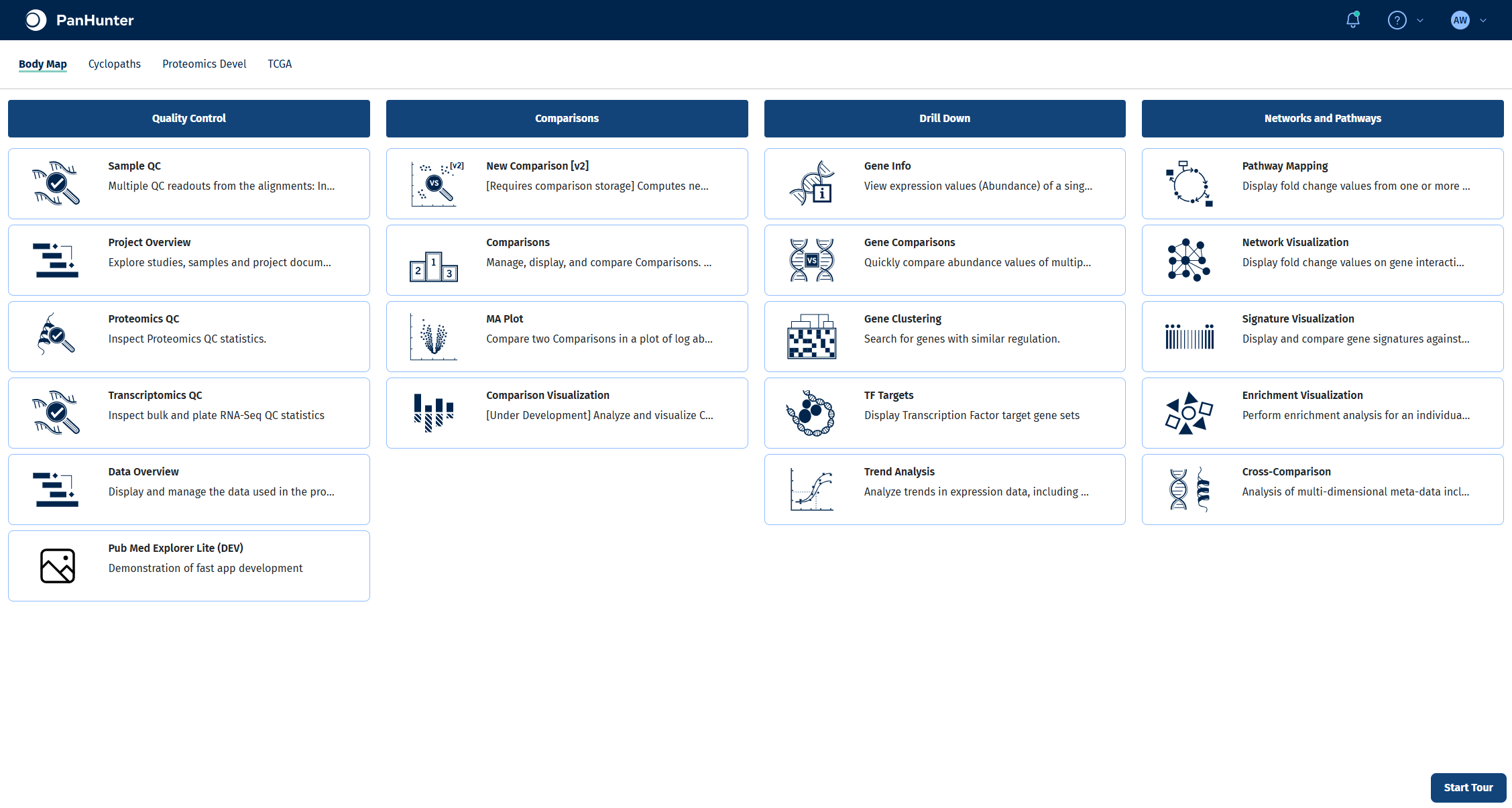
All steps up to the calculation happen in the New Comparison [v2] app. Open it from the start page of your project.
Selecting samples in the Sample Selector panel on the left defines which samples every tab of the app works with, including the comparison you calculate later. Narrowing the selection down to exactly the samples of your question keeps plots readable and makes sure the statistical model is only fitted on relevant samples.
- In Studies, select Yu2014. The panel shows how many samples were loaded.
- In Add a new modifier, choose Filter categ. and click +.
- In the new filter, set Filter to Tissue, keep Include and select Liver in Values.
- Add a second Filter categ. modifier with Filter set to Age and Values set to 6 and 104.
For more on modifiers, see the Sample Selector documentation.
Check your result
The Sample Selector panel reads Loaded 15 out of 316 samples and shows the two filters Tissue: Liver and Age: 6, 104.
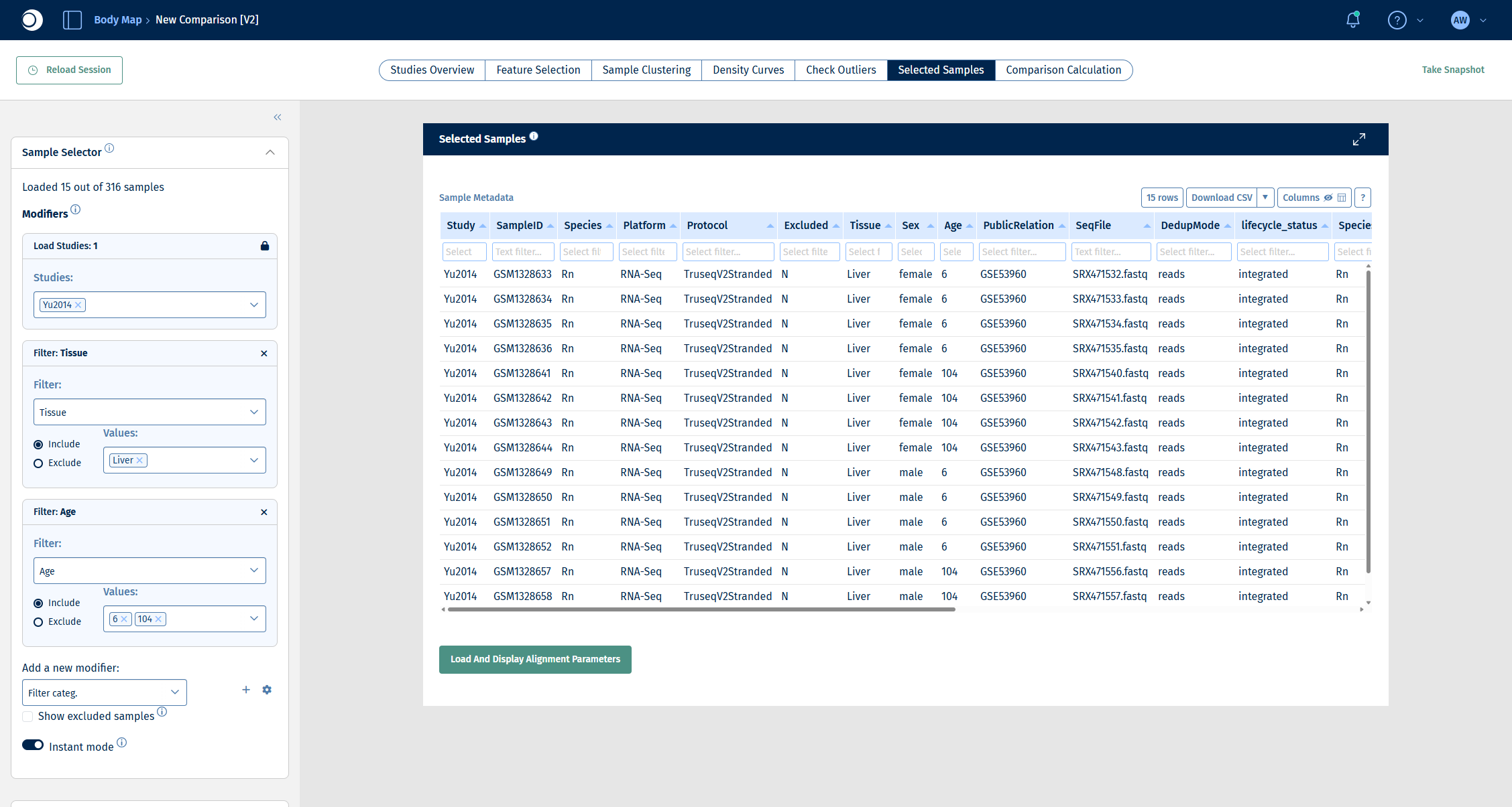
Note: The Studies Overview tab summarizes the whole study and does not reflect the filters. Use the Selected Samples tab to see the samples that are actually selected.
Step 2: Explore how the samples group
Before calculating a comparison, checking how the samples relate to each other tells you which factors drive the biggest differences in your data. Factors with a visible effect that are not the subject of your question are candidates for the comparison formula, so that the model can account for them.
- Open the Sample Clustering tab. It shows a PCA of the selected samples.
- In the left sidebar, scroll down to Plot Options.
- Set Color to Sample meta data and pick a metadata column, for example Sex.
- Switch the color column to Age and set Symbol to Sample meta data and Sex.
Try other columns as well: coloring by different metadata is the quickest way to spot batch effects or unexpected groupings. For all options, see Plot Options panel and Dimension Reduction panel.
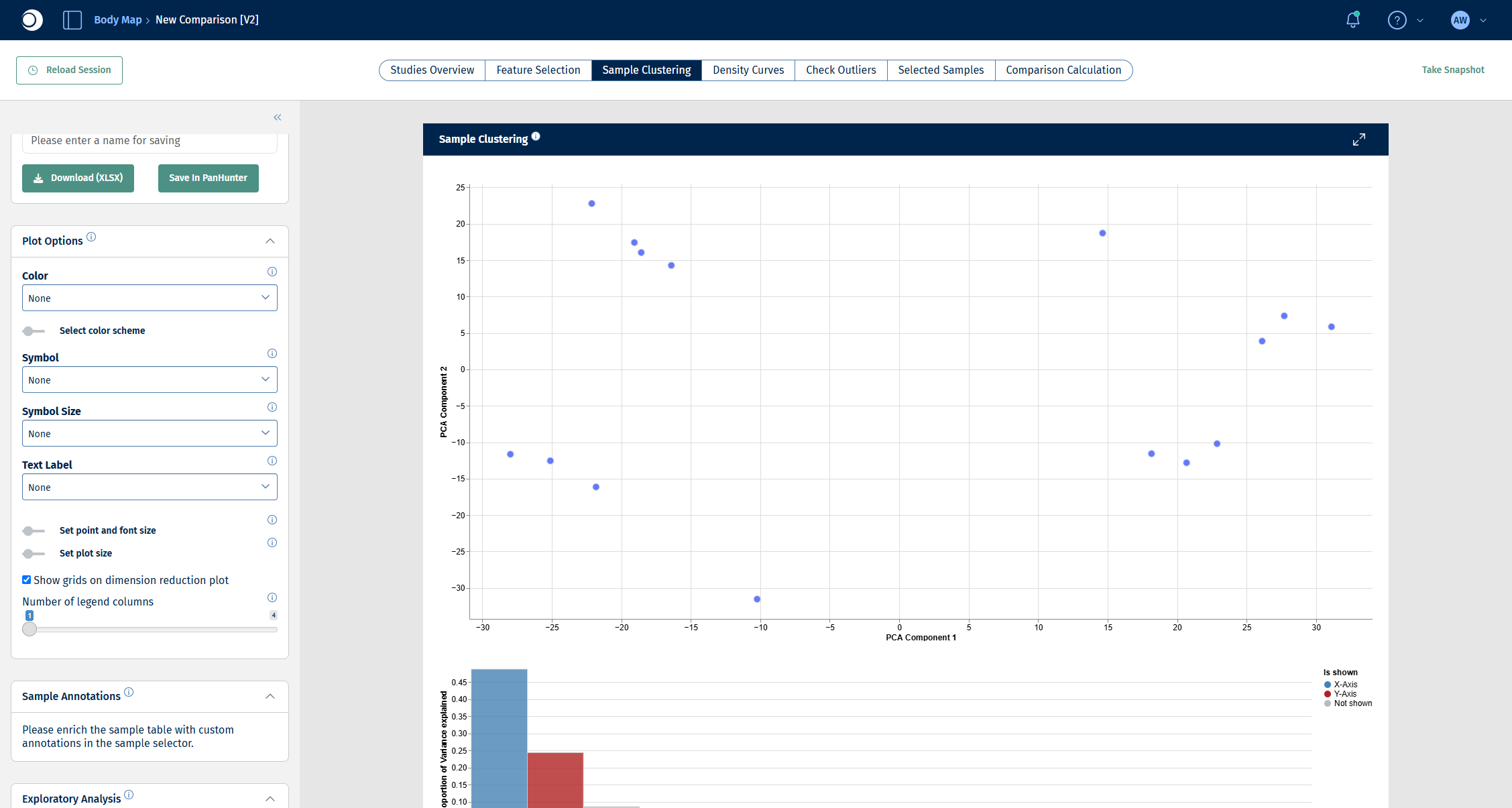
Check your result: PCA without coloring
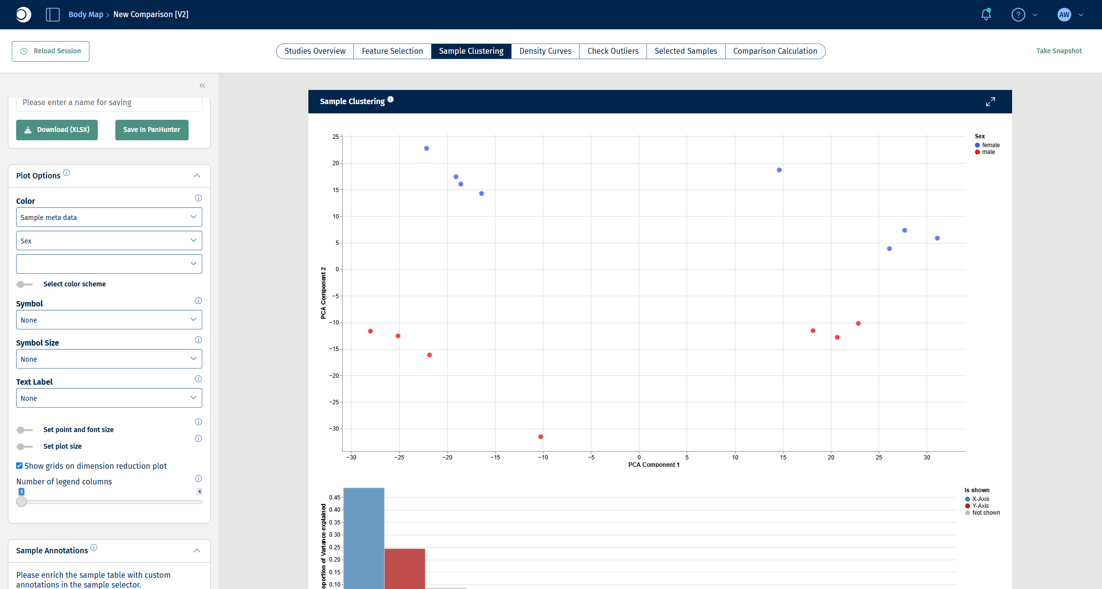
Check your result: PCA colored by sex
The samples split along the second principal component (y-axis) by sex.
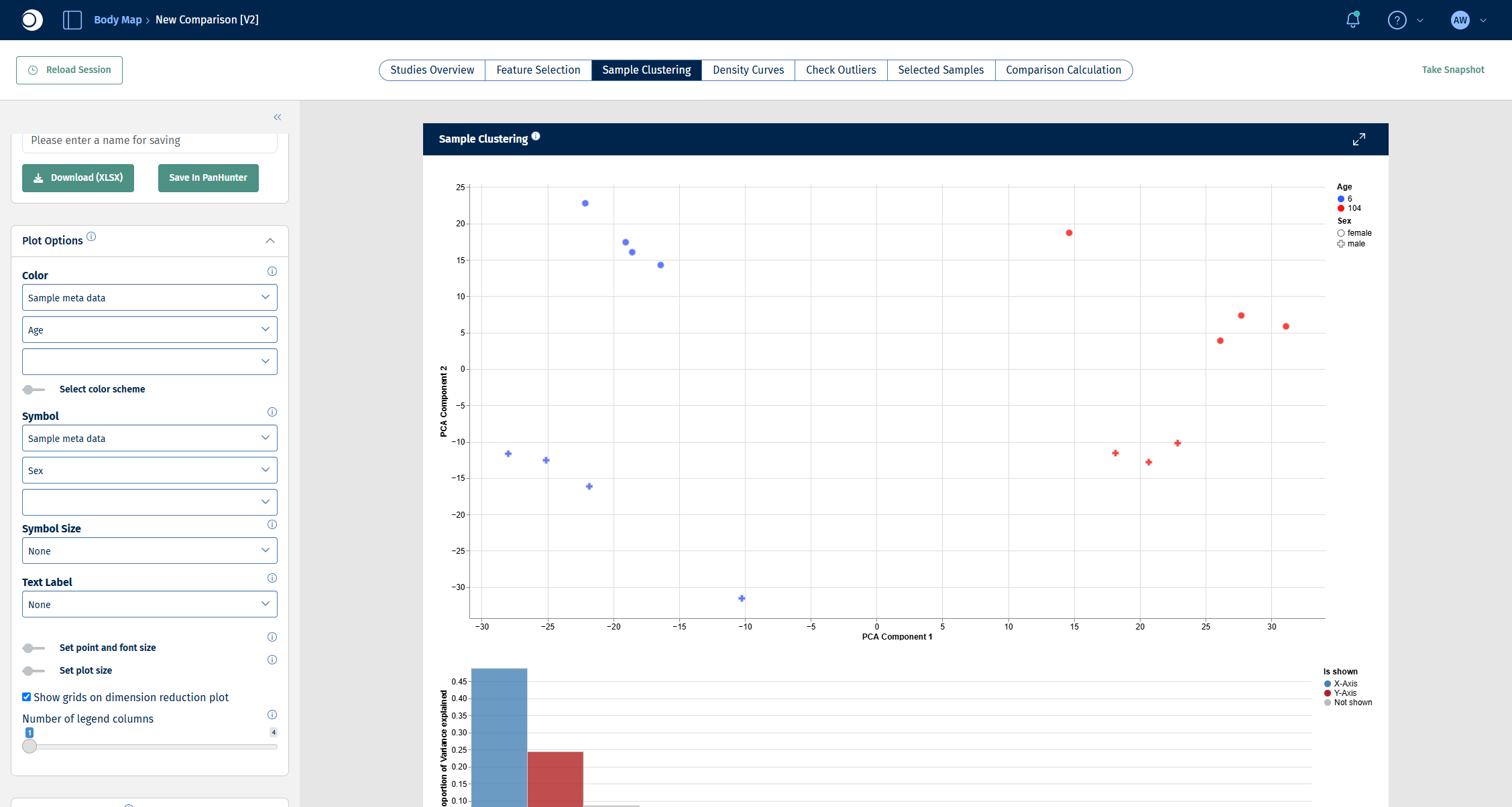
Check your result: PCA colored by age, symbols by sex
The samples split along the first principal component (x-axis) by age: 6-week samples on the left, 104-week samples on the right. Age explains the largest part of the variance, sex the second largest. That is why the comparison in the next step includes both factors.
Step 3: Set up and validate the comparison
The Comparison Calculation tab defines which groups are compared and how. A single run can create many comparisons at once; for this guide one comparison is enough. All fields are described in detail in New Comparison: Comparison Calculation.
- Open the Comparison Calculation tab.
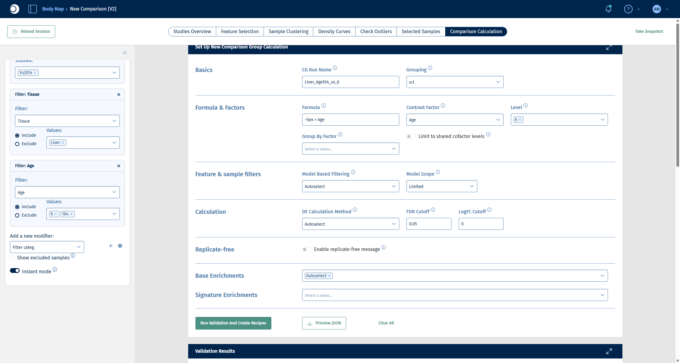
- Under Basics, enter a CG Run Name, for example
Liver_Age104_vs_6, and keep Grouping at n:1. The name must be unique in the project; in the screenshots of the later steps the run is called Guide_Liver_Age104_vs_6. - Under Formula & Factors:
- enter the Formula
~Sex + Age. Including Sex lets the model account for the sex difference you saw in step 2, so that the comparison isolates the effect of age. - set Contrast Factor to Age.
- set Level to 6. The level you select here is the reference (denominator); the remaining level, 104, becomes the numerator.
- Leave Feature & sample filters, Calculation and Base Enrichments at their defaults (Autoselect).
- Click Run Validation And Create Recipes.
Important: Factor names in the formula are case-sensitive and must match the metadata column names exactly.
Check your result: set-up
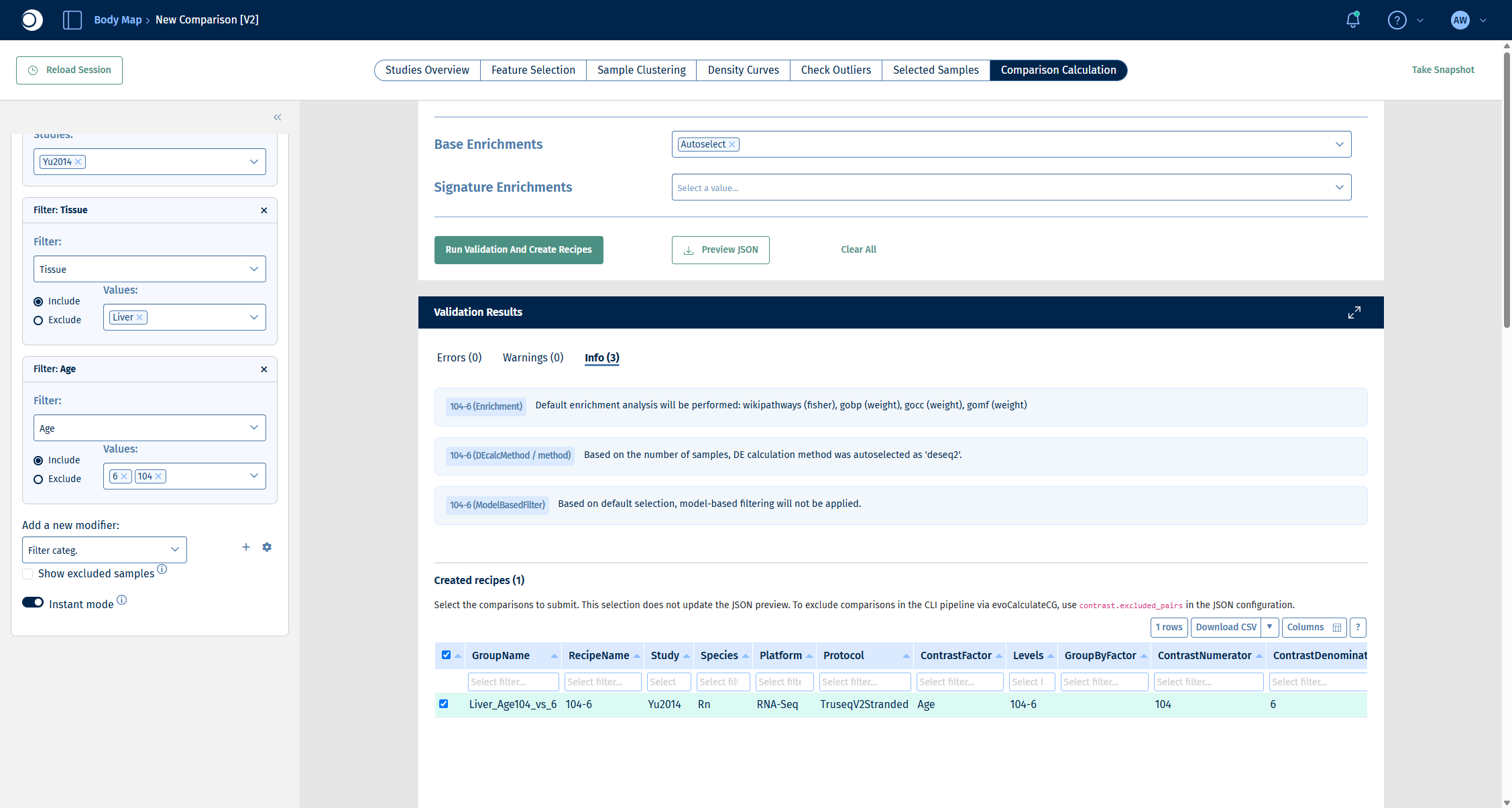
Validation checks your set-up without calculating anything. The Validation Results section lists errors, warnings and info messages, followed by the comparisons (recipes) that would be calculated.
Check your result: validation
- Errors (0) and Warnings (0).
- Info (3): default enrichment analysis with wikipathways (fisher), gobp, gocc and gomf (weight); DE method autoselected as deseq2 based on the number of samples; no model-based filtering.
- Created recipes (1): one recipe 104-6 with 7 numerator and 8 denominator samples.
The wikipathways (fisher) enrichment in the info messages is a pathway over-representation analysis that is calculated together with the comparison. You will explore enrichments interactively in step 5.
Step 4: Run the calculation and inspect the DE results
- Scroll down to the recipe table, make sure the recipe is checked and click Submit Calculation To SLURM.
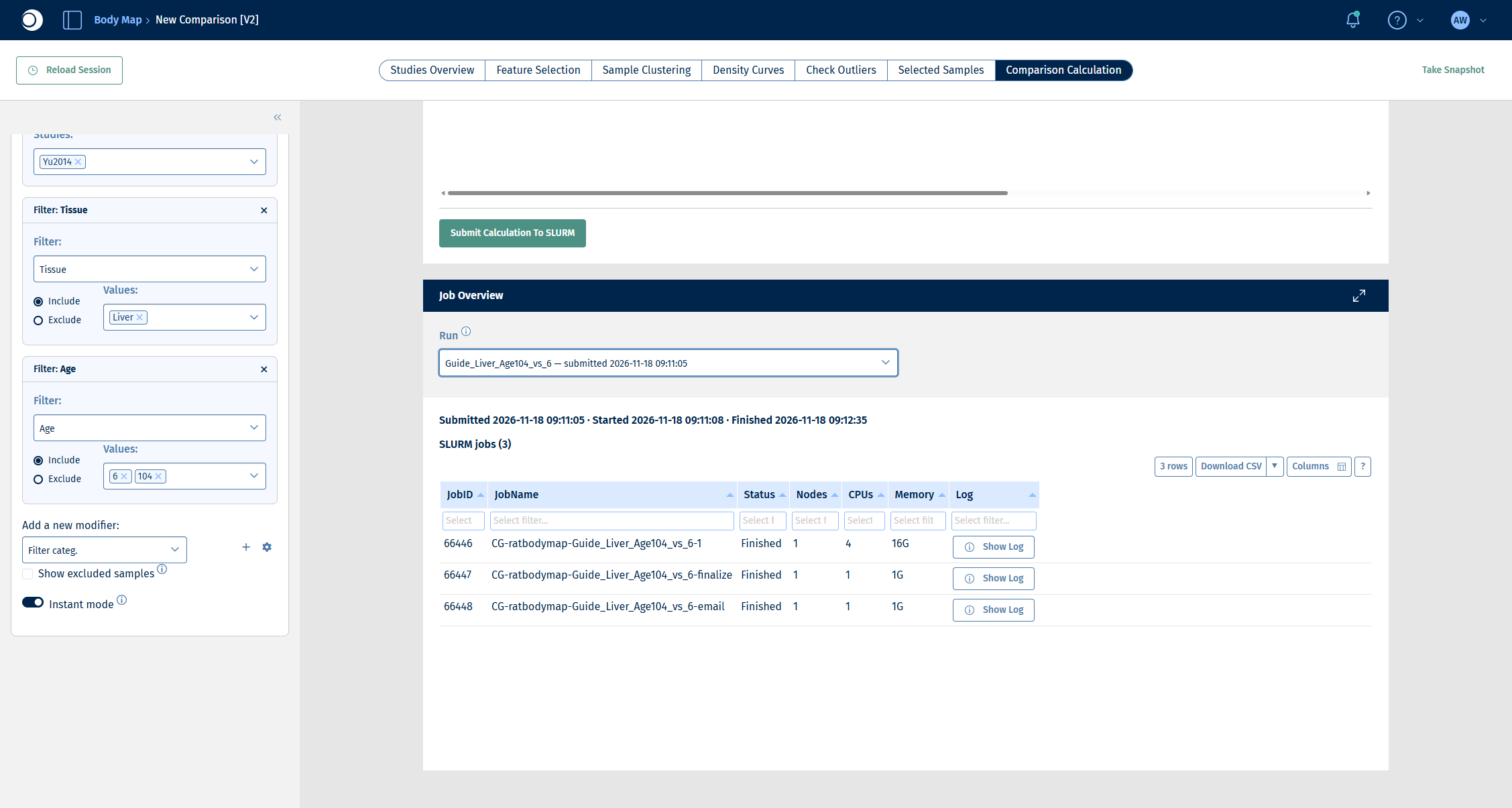
- Follow the progress in the Job Overview section. Select your run in Run. A run consists of three jobs: the calculation itself, a finalize job and an email job. For this example the whole run takes about two minutes.
Check your result: job overview
All three jobs show the status Finished.
When the run has finished, open the Comparisons app from the start page.
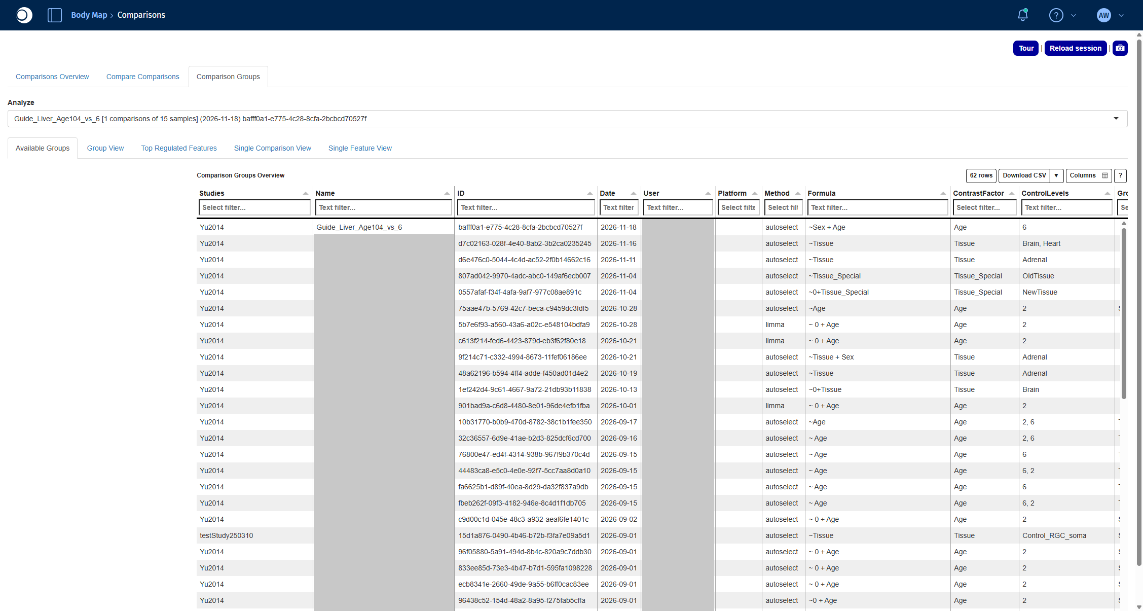
- Open the Comparison Groups tab. Comparisons calculated in the Comparison Calculation tab are listed here, grouped by run. In Analyze, select your run.
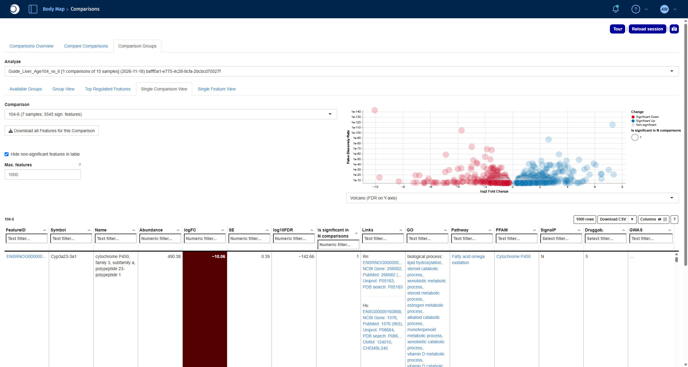
- Open the Single Comparison View tab and select the comparison 104-6 in Comparison.
The volcano plot shows the fold change (x-axis) against the significance (y-axis) of every gene; red genes are significantly down, blue genes significantly up in old compared to young liver. The table below lists the significant genes with their fold change, FDR and links to external databases. For all functions of the app, see Comparisons.
Check your result: Comparison Groups
Check your result: DE results
The comparison reads 104-6 (7 samples; 3545 sign. features). The most strongly changed gene is Cyp3a23/3a1, a cytochrome P450 enzyme, with a log2 fold change of about −10.
Step 5: Find over-represented pathways
An over-representation analysis tests whether the differentially expressed genes contain more members of a pathway than expected by chance. The Enrichment Visualization app runs this test for any gene set collection and shows the results as plots and tables.
- Open the Enrichment Visualization app from the start page.
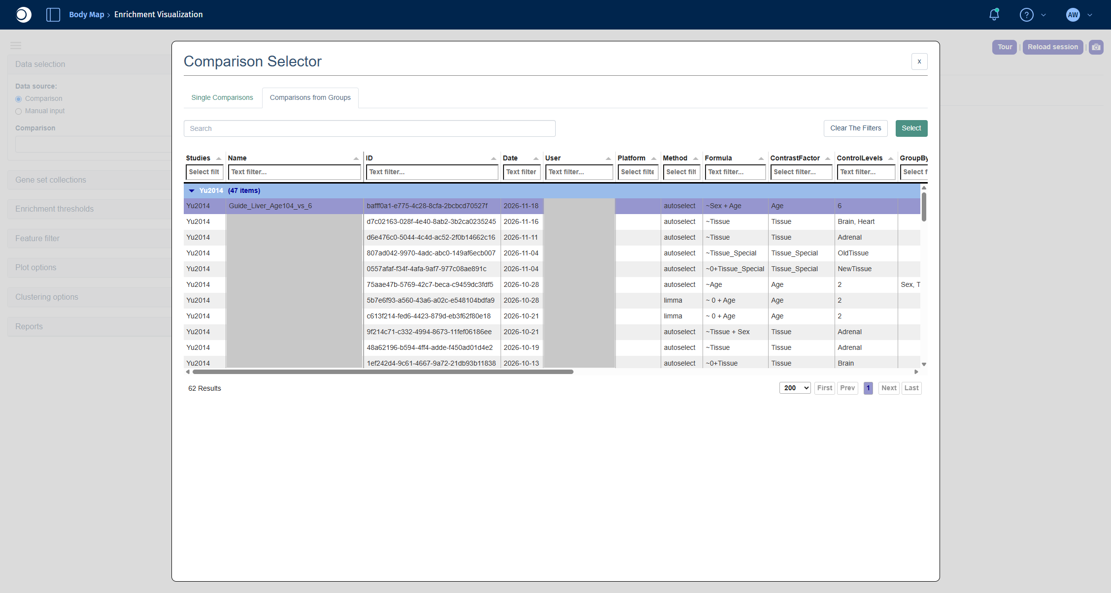
- Under Data selection, keep Comparison as data source and click into the Comparison field. The Comparison Selector opens.
- Open the Comparisons from Groups tab, select your run and click Select. In the next view, select the comparison 104-6 and click Select again.
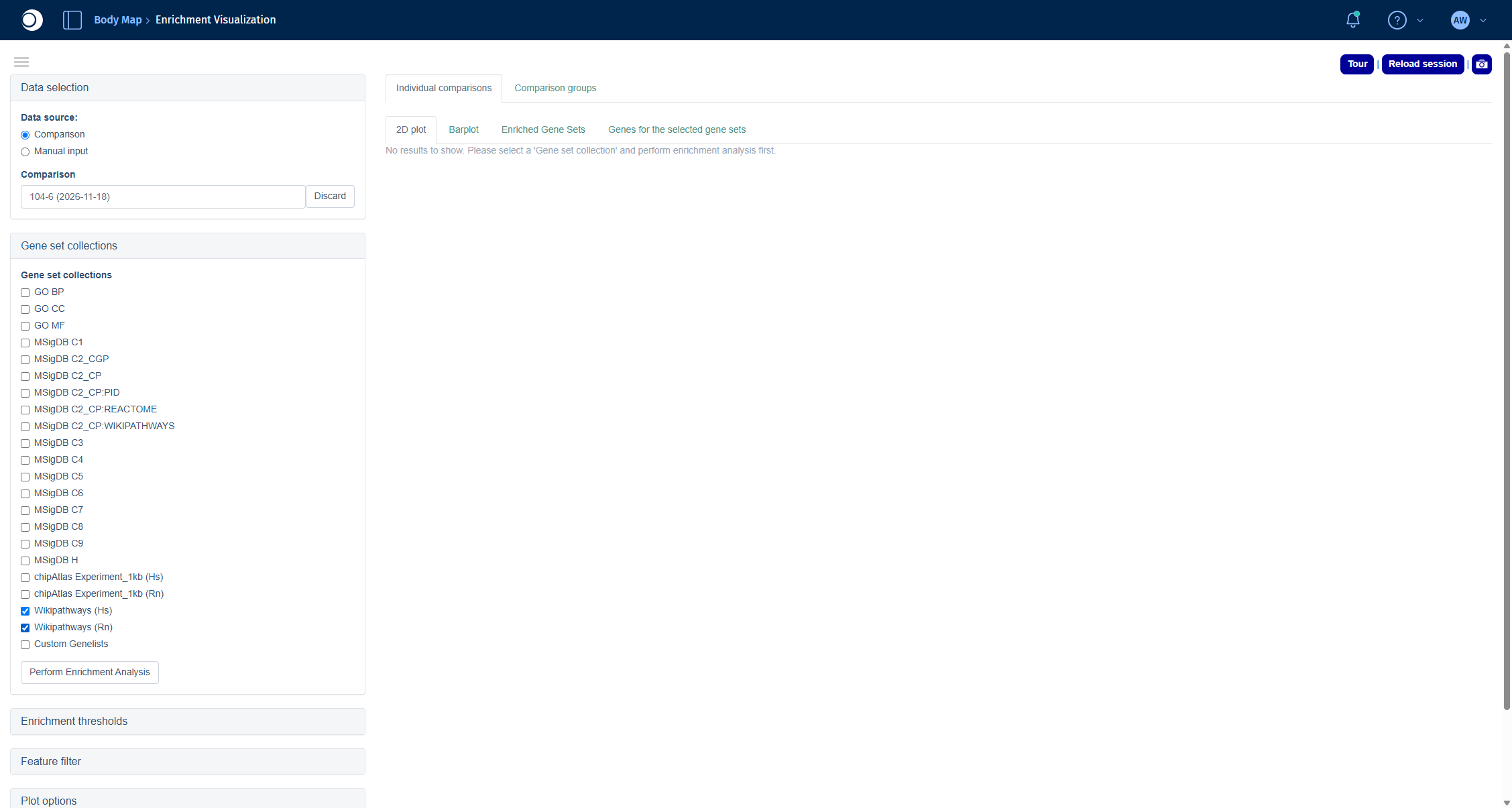
- Open Gene set collections and check Wikipathways (Hs) and Wikipathways (Rn).
- Click Perform Enrichment Analysis.
Recommendation: For non-human data, always add the human collection (here Wikipathways (Hs)) to the collection of your species. Human pathways are annotated much more comprehensively, and PanHunter maps your genes to their human orthologs. In this example, Wikipathways (Rn) alone finds only two enriched pathways, together with Wikipathways (Hs) it finds 64.
Check your result: Comparison Selector
Check your result: gene set collections
The results are spread over four tabs:
- Enriched Gene Sets: the table of enriched pathways with the number of genes, the number of significant genes up and down, p-value and FDR.
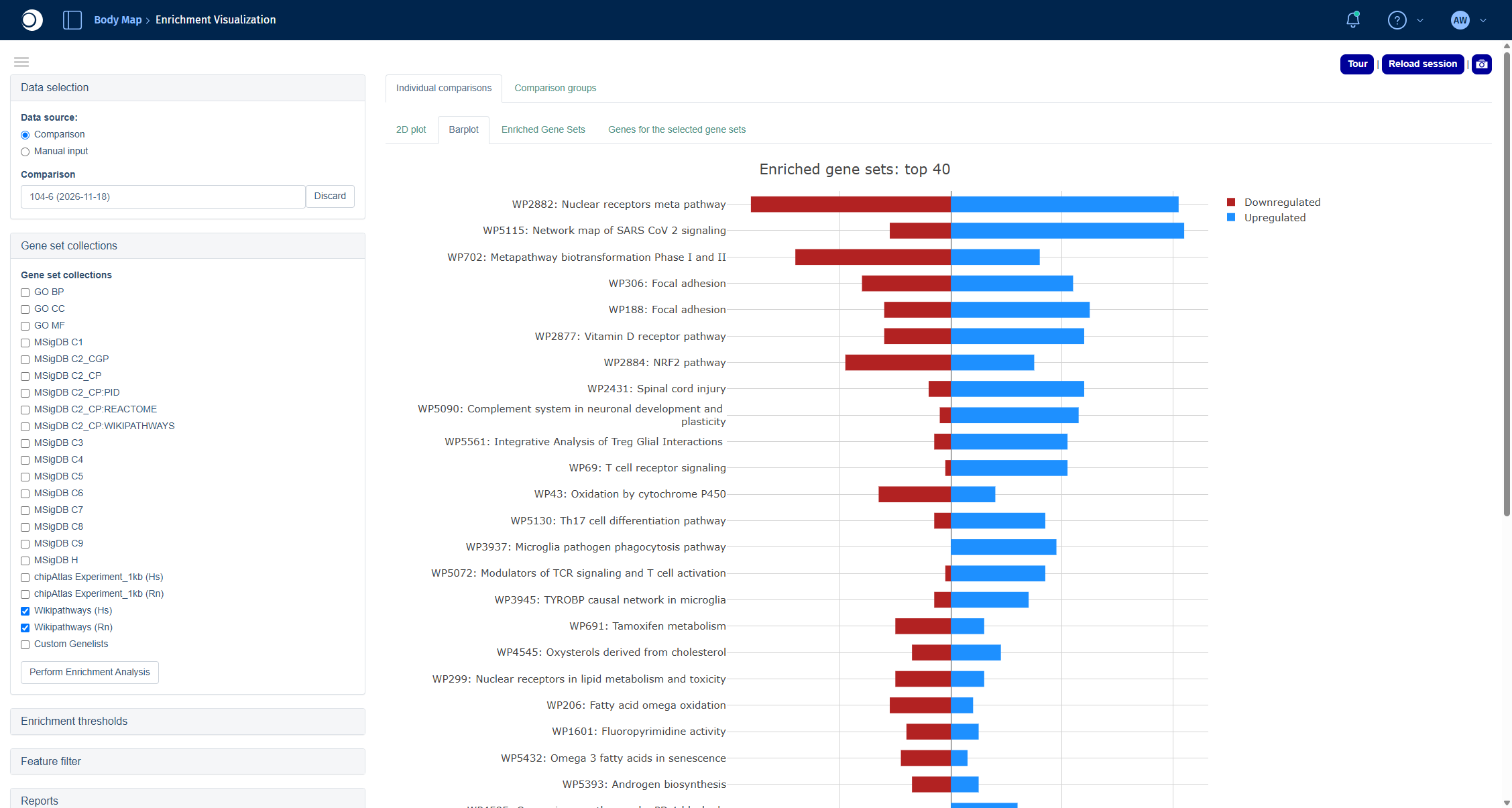
- Barplot: the top 40 pathways with the number of up- and downregulated genes.
- 2D plot: pathways arranged by similarity of their gene content.
- Genes for the selected gene sets: the genes of the pathways you select in one of the other tabs.
For all options, including thresholds and filters, see Enrichment Visualization.
Check your result: enriched pathways
The table contains 64 pathways. Among the top hits are Nuclear receptors meta pathway, Tamoxifen metabolism, Fatty acid omega oxidation and Metapathway biotransformation Phase I and II, which points to changes in the drug and lipid metabolism of the aging liver.
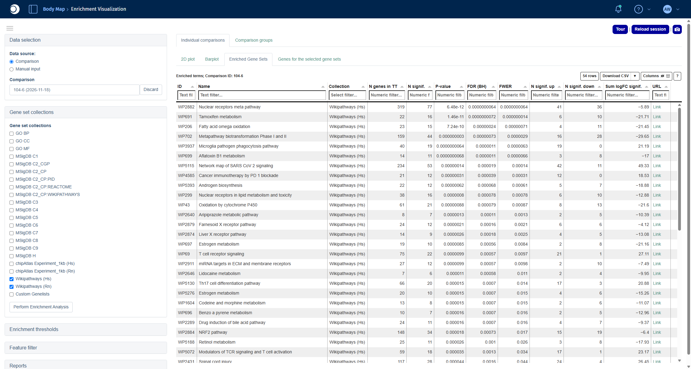
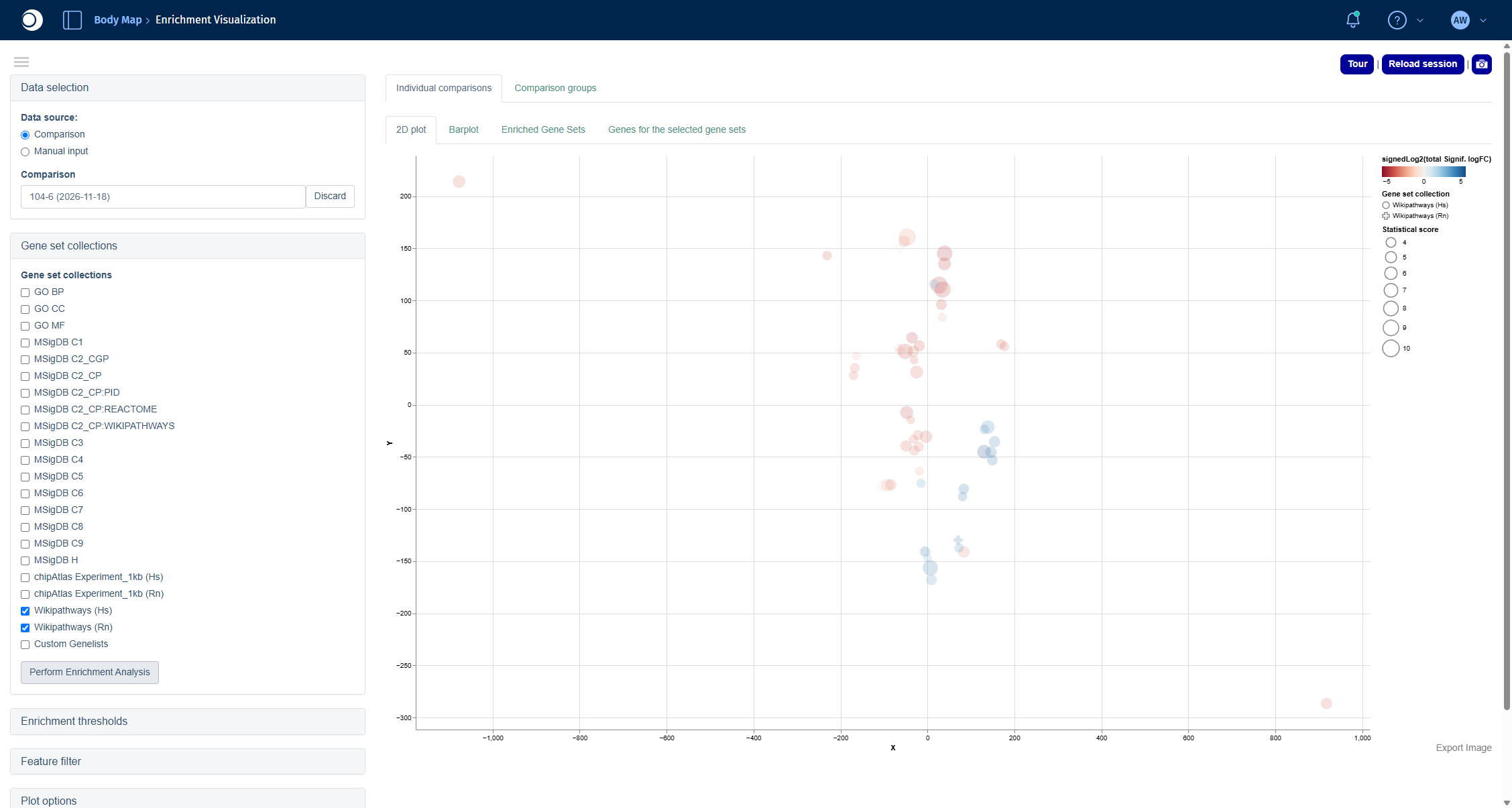
Check your result: 2D plot
Each circle is an enriched pathway. Pathways that share many genes lie close to each other; the color shows whether the significant genes of a pathway are mostly down (red) or up (blue), the size shows the statistical score.
Check your result: barplot
Step 6: Look at a single pathway
The Pathway Mapping app draws a pathway and colors each gene by its fold change, so you can see which parts of the pathway change and in which direction.
- Open the Pathway Mapping app from the start page.
- Click into Comparison 1 and select your comparison in the Comparison Selector the same way as in step 5.
- In Select pathway, type part of the pathway name, for example
omega oxidation, and select Fatty acid omega oxidation (Hs, WP206).
For coloring options and the table view, see Pathway Visualization.
Check your result: pathway
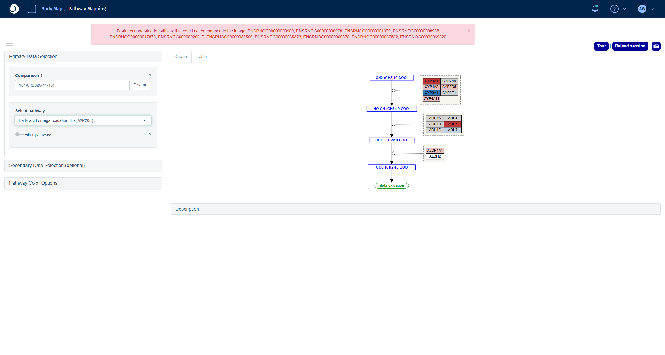
The pathway shows the conversion of fatty acids along with the enzymes catalyzing each step. Red boxes are downregulated, blue boxes upregulated genes in old compared to young liver.
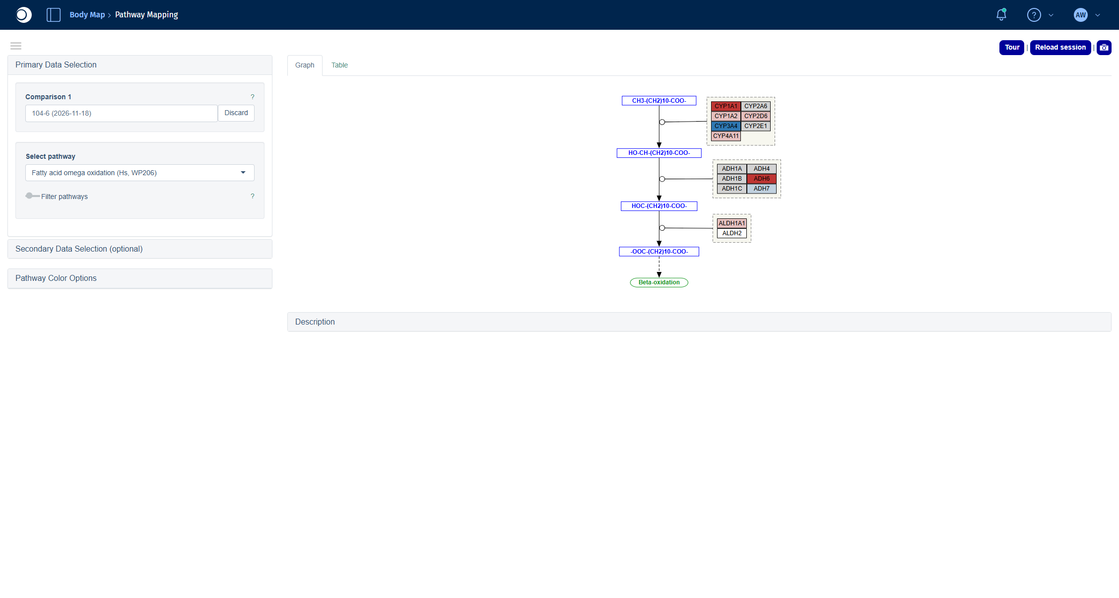
Troubleshooting
My new comparison does not show up in the Comparisons app.
Comparisons calculated in the Comparison Calculation tab are listed in the Comparison Groups tab, not in Comparisons Overview. In apps with a Comparison Selector, use the Comparisons from Groups tab. Make sure the run is finished in the Job Overview.Pathway Mapping shows a red message about features that could not be mapped to the image.
The pathway contains genes of your comparison that have no counterpart in the pathway drawing, for example because the drawing is based on human genes. The message lists their IDs. The pathway is still drawn correctly for all mapped genes.
The Enrichment Visualization shows the message Assigning random coordinates.
The 2D plot needs a minimum number of enriched gene sets. If fewer pass the thresholds, the pathways are placed randomly. Add more collections (see the recommendation in step 5) or relax the Enrichment thresholds.Next steps
- Compare your comparison with other comparisons in Compare Comparisons.
- Look at the genes of an enriched pathway in their interaction network with Network Visualization.
- Check which transcription factors could explain the expression changes with TF Targets.
2 - Find what drives the clustering of your samples
Find out which metadata and which genes explain how your samples group, spot and inspect outliers, and learn which biology the driving genes represent.
Before you calculate any comparison, it pays to understand how your samples relate to each other. This guide shows you how to answer three questions with the New Comparison [v2] and Enrichment Visualization apps:
- Which metadata, for example tissue, age or sex, explains how the samples group?
- Which genes drive this grouping, and which biology do they represent?
- Are there samples that do not fit, and what is wrong with them?
You will:
- load a study and look at a PCA of all samples,
- let the Exploratory Analysis rank metadata and genes by how well they explain the PCA,
- find an outlier sample and check why it is an outlier,
- repeat the analysis for a single tissue and
- run an over-representation analysis on the genes that drive the grouping.
The guide takes about 30 minutes, most of it waiting for calculations. You do not need to calculate a comparison.
Before you start
- Access: You need access to a PanHunter project with the apps New Comparison [v2] and Enrichment Visualization.
- Example data: The guide uses the study Yu2014, a public rat body map (GSE53960) with eleven tissues from rats aged 2, 6, 21 and 104 weeks, both sexes. If your project does not contain Yu2014, follow the same steps with your own study.
- Background: The methods behind the steps are explained in Dimensionality reduction, Exploratory analysis and Enrichment analysis.
Step 1: Load the study
Open the New Comparison [v2] app from the start page of your project. The Sample Selector panel on the left defines which samples all tabs of the app work with.
- In Studies, start typing
Yu20 and select Yu2014. - Do not add any filter yet: this time you want to see all samples.
Check your result
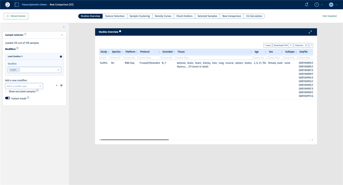
The Sample Selector reads Loaded 315 out of 318 samples. Three samples are excluded by default because they failed quality control. The Studies Overview tab lists the eleven tissues, the four age groups and both sexes.
Step 2: Look at the PCA of all samples
- Open the Sample Clustering tab. It shows a PCA of the selected samples, with the explained variance per principal component in the bar chart below.
- In the left sidebar, open Plot Options.
- Set Color to Sample meta data and select Tissue. Set Symbol to Sample meta data and select Sex.
- Switch the color column to Age.
For all display options, see Plot Options panel.
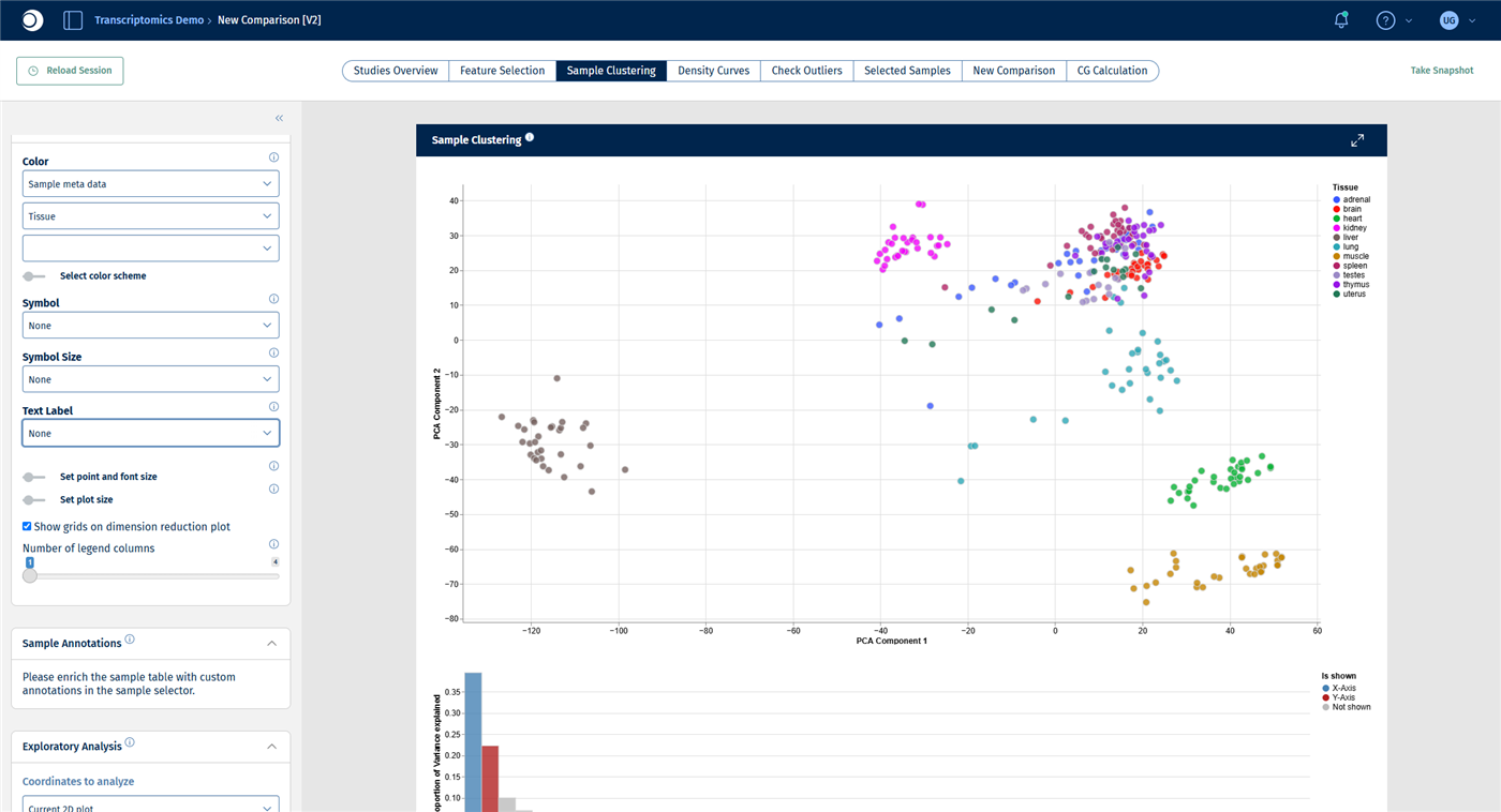
Check your result: PCA colored by tissue
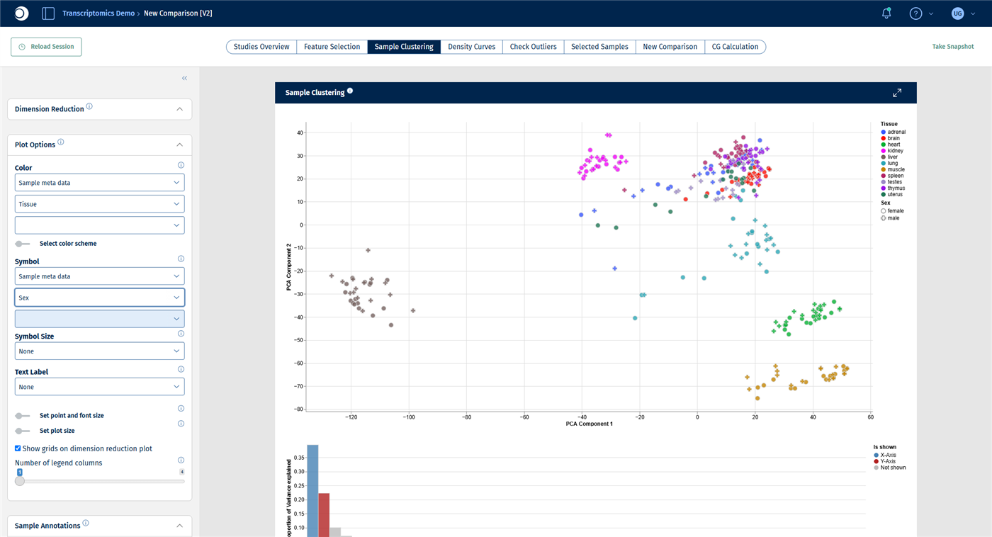
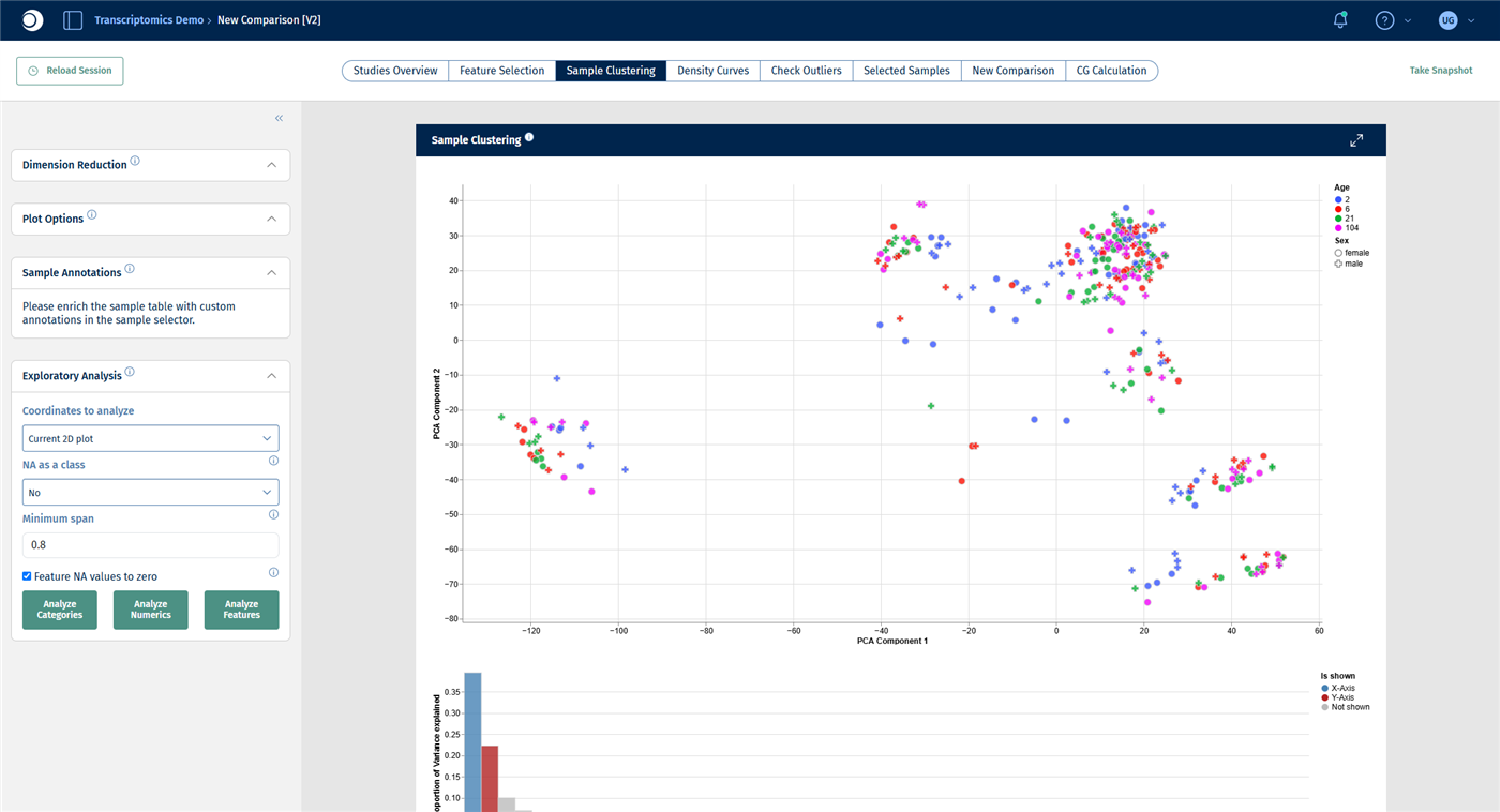
Most tissues form their own cluster. Liver lies far to the left, kidney, lung, heart and muscle are clearly separated, while brain, spleen, thymus, testes, uterus and adrenal gland overlap more. The first two principal components explain about 39 % and 22 % of the variance.
Check your result: PCA colored by age
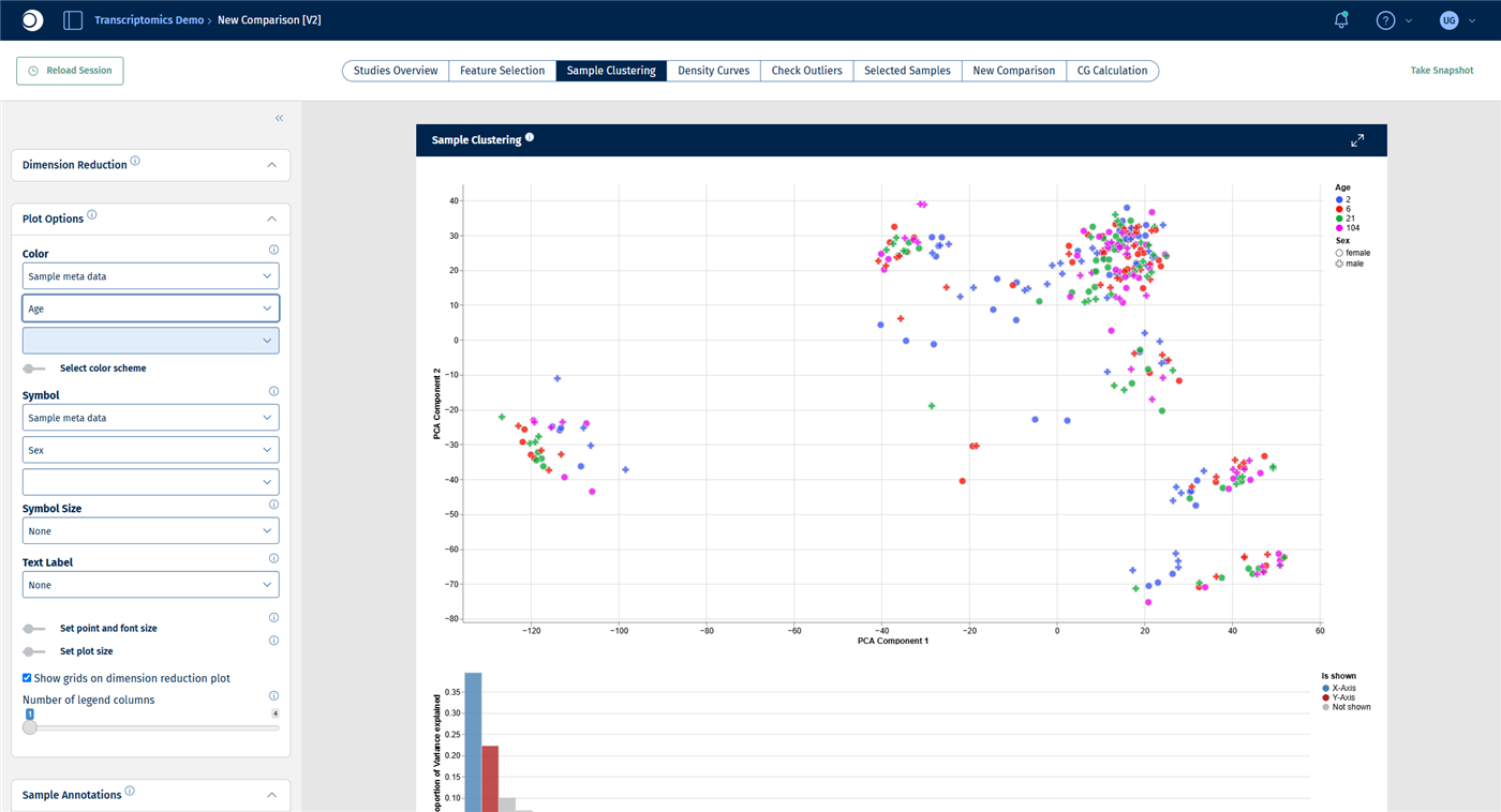
The age groups are mixed within every tissue cluster. Across all tissues, age has no visible effect on the first two principal components.
Looking at colors works well for a few metadata columns. The next step does the same systematically for all columns and all genes.
The Exploratory Analysis panel tests which metadata columns and which features (here: genes) are associated with the current plot. For a detailed description of all settings, see Exploratory analysis panel.
- In the left sidebar, collapse Dimension Reduction and Plot Options by clicking their headers, so that the Exploratory Analysis panel becomes visible.
- Keep Coordinates to analyze at Current 2D plot and the other settings at their defaults.
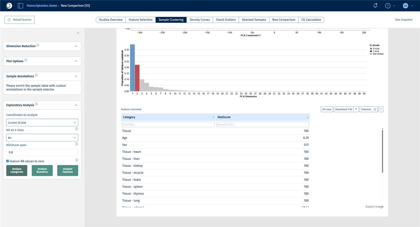
- Click Analyze Categories. After a few seconds, the result appears as a table below the bar chart.
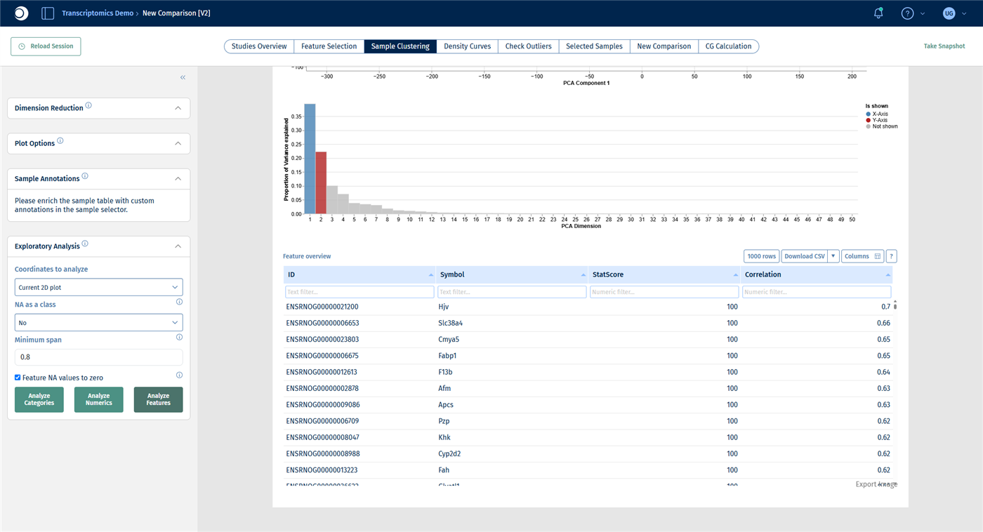
- Click Analyze Features. The table now lists genes.
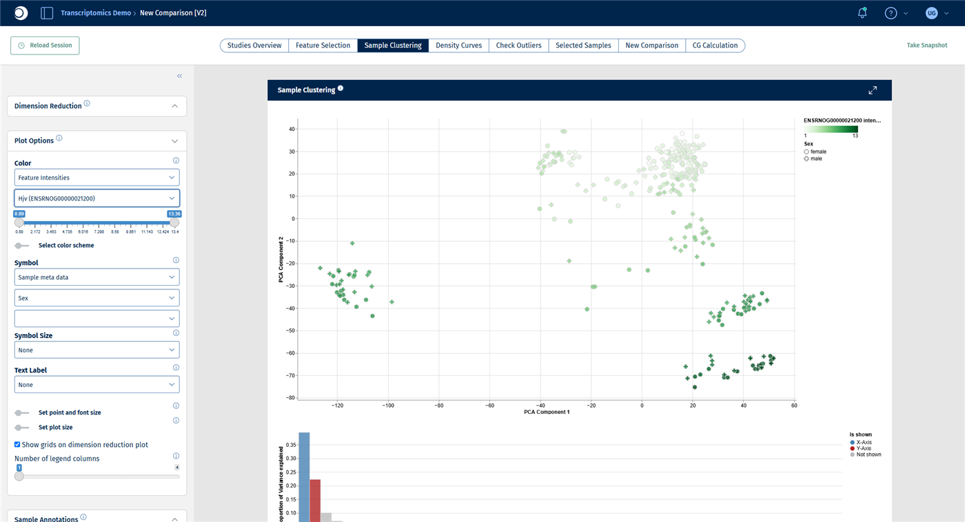
- In Plot Options, set Color to Feature Intensities and type the symbol of the top gene, here
Hjv, into the feature field.
Check your result: settings
Check your result: categories
The table lists each metadata column and each of its levels with a StatScore: the higher the score, the better the column or level explains the position of the samples in the plot. Tissue reaches the maximum score of 100, while Age (0.29) and Sex (0.11) hardly explain anything. This confirms what you saw in step 2.
Check your result: features
The genes are sorted by their Correlation with the plot coordinates. The top genes, such as Hjv, Slc38a4, Fabp1 and F13b, are mostly liver genes. They explain why the liver samples are so far away from all other tissues. Colored by Hjv, the liver cluster is clearly darker than the rest.
Note: Analyze Numerics answers No numeric variables found in sample table. for this study. Although age is a number, Yu2014 stores it as four groups (2, 6, 21 and 104 weeks), that is, as a category. That is why age appears in the results of Analyze Categories, with one row per age group. In studies with a numeric column, for example age in years or a quality score, use Analyze Numerics to find out whether the column follows the plot.
Step 4: Find and inspect an outlier
Public data is not perfect, and neither is your own. A sample that sits apart from the other samples of its group can be a biological extreme, but also a technical problem such as contamination or a sample mix-up. Such samples can distort every analysis that follows, so check them before you calculate comparisons.
- Color the PCA by Tissue again. Look for samples that lie far away from the cluster of their own tissue. In Yu2014, a few lung samples lie well below the lung cluster.
- To find out which samples they are, set Text Label in Plot Options to Sample meta data and SampleID, or hover over a point. The most isolated lung sample is GSM1328601.
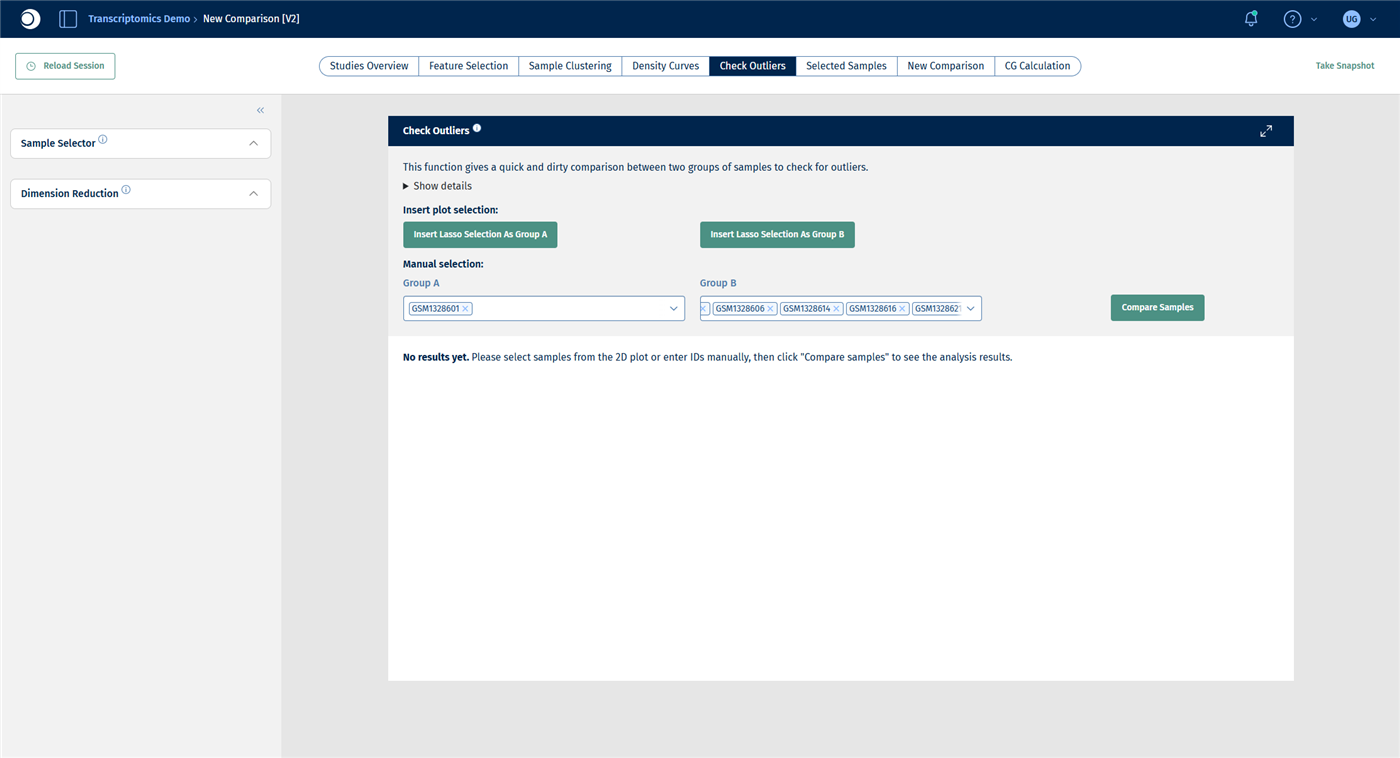
- Open the Check Outliers tab. Under Manual selection, type
GSM1328601 into Group A and press Enter. Add some other lung samples to Group B, for example GSM1328604, GSM1328606, GSM1328614, GSM1328616, GSM1328621 and GSM1328627. - Click Compare Samples.
Instead of typing sample IDs, you can also select points in the plot with the lasso and click Insert Lasso Selection As Group A or B. For details, see New Comparison: Check Outliers.
Check your result: outlier in the PCA
Check your result: groups
Check your result: outlier table
The Custom outlier table lists the genes with the largest differences between the two groups. At the top are Ces2j, Akr1d1, Slco1b2, Serpina3c, Cyp1a2 and Cyp7a1: genes that are typically expressed in the liver, not in the lung. The “lung” sample GSM1328601 most likely contains liver tissue or was mixed up.
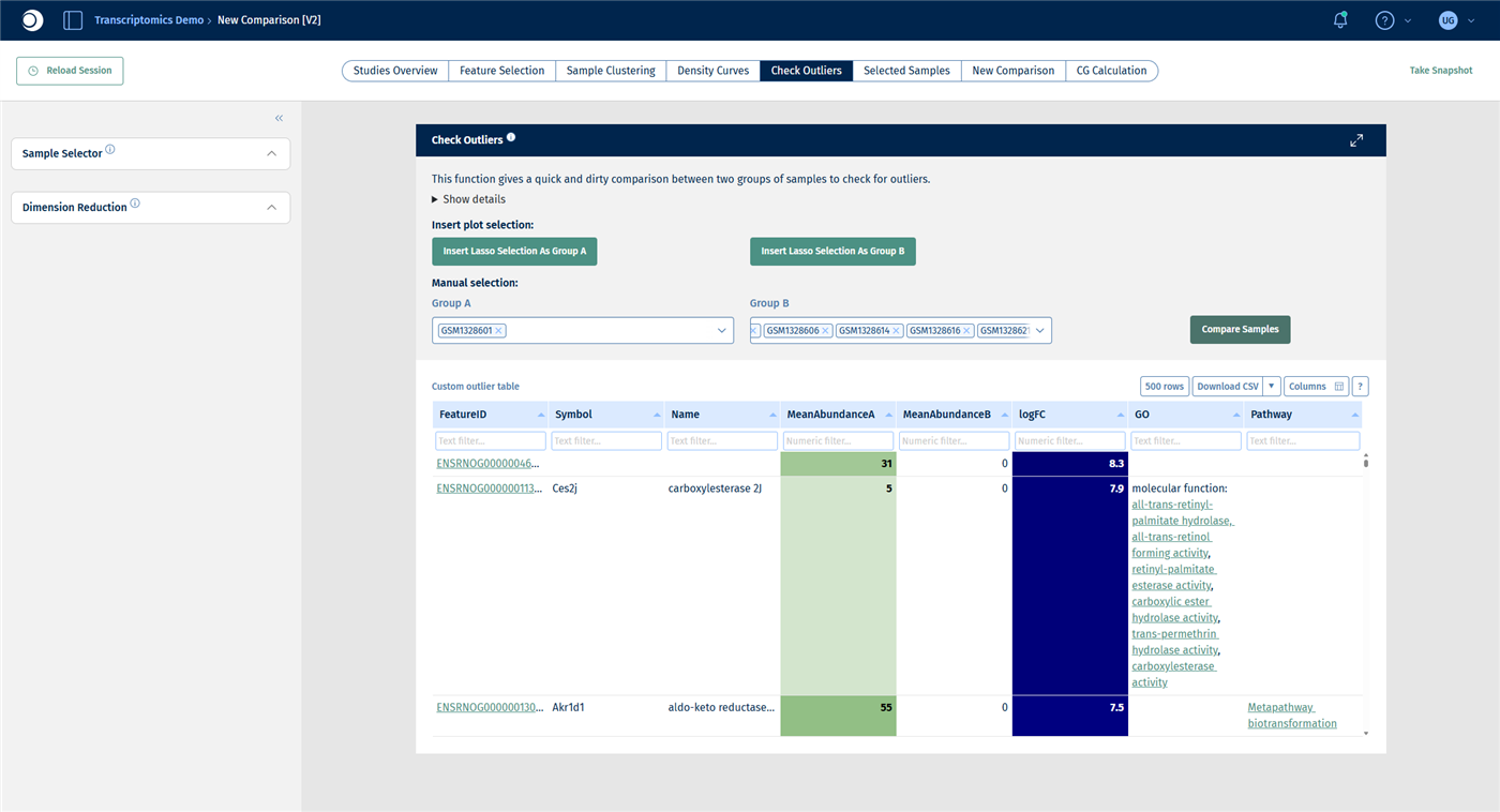
Important: Check Outliers is a quick comparison without any statistical test. Genes with very low counts can reach large fold changes by chance. Use it to understand an outlier, not to find differentially expressed genes.
Once you have decided that a sample should not be used, remove it from the selection:
- In the Sample Selector, add a Filter categ. modifier.
- Set Filter to SampleID, select Exclude and enter
GSM1328601 in Values.
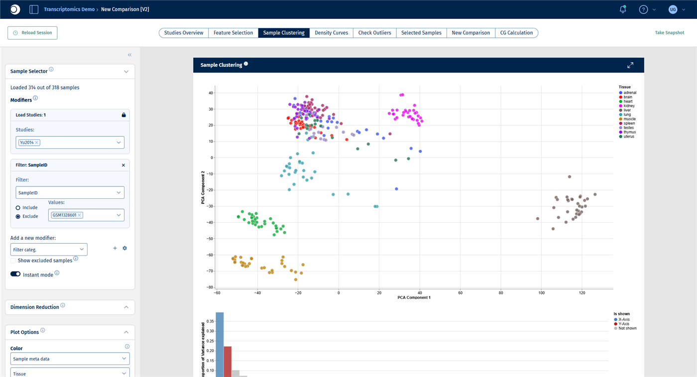
Check your result: sample excluded
The Sample Selector reads Loaded 314 out of 318 samples and the PCA is recalculated. Do not be surprised if the plot appears mirrored: the sign of a principal component is arbitrary. A few other lung samples still lie apart; check them the same way before you exclude them.
Step 5: Repeat the analysis for one tissue
Within a tissue, smaller effects such as age and sex become visible that are hidden by the large differences between tissues.
- Keep the SampleID filter from step 4; it does not affect the liver samples.
- Add a Filter categ. modifier with Filter set to Tissue, Include and Values set to liver.
- In the Sample Clustering tab, set Color to Age and Symbol to Sex.
- In the Exploratory Analysis panel, click Analyze Categories and then Analyze Features.
Check your result: liver PCA
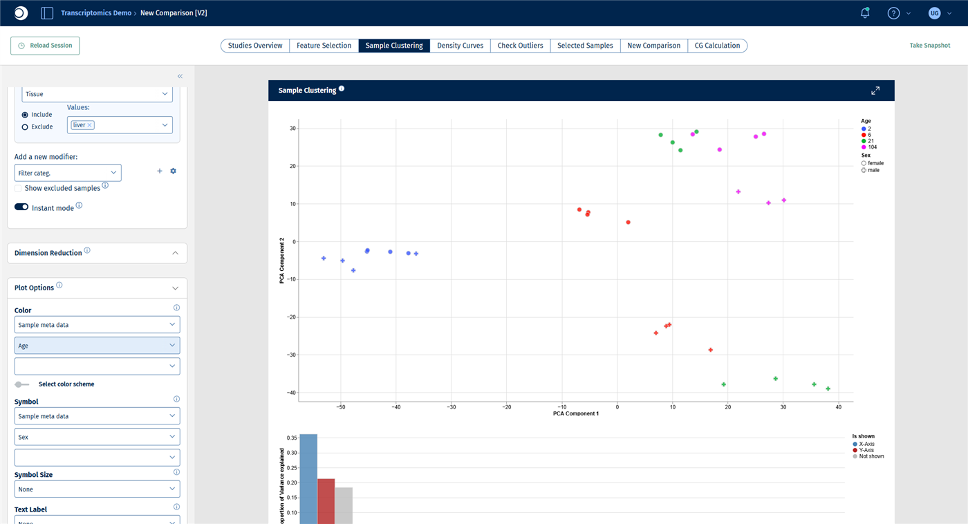
The selection contains 31 liver samples. The first principal component separates the samples by age, from 2-week-old rats on the left to 104-week-old rats on the right. The second principal component separates females from males.
Check your result: categories
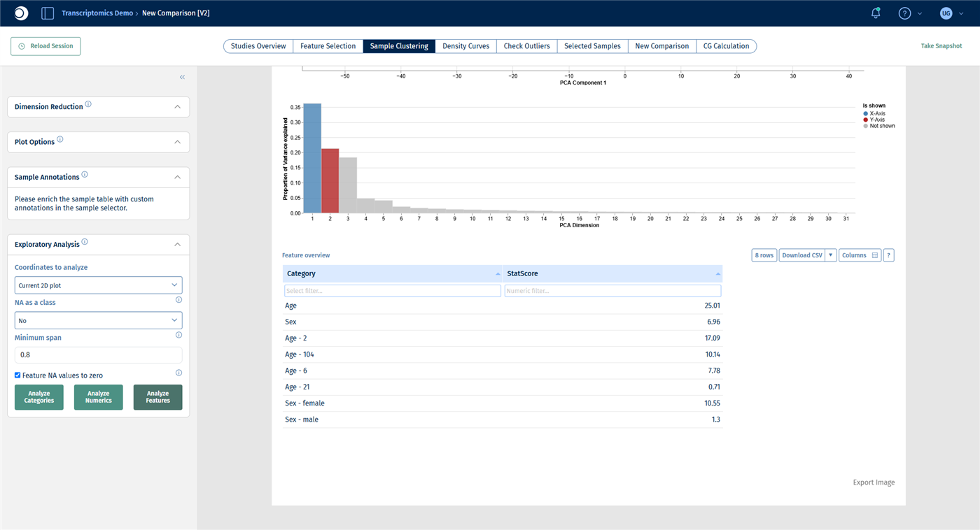
Now Age ranks first (StatScore about 25), followed by Sex (about 7).
Check your result: features
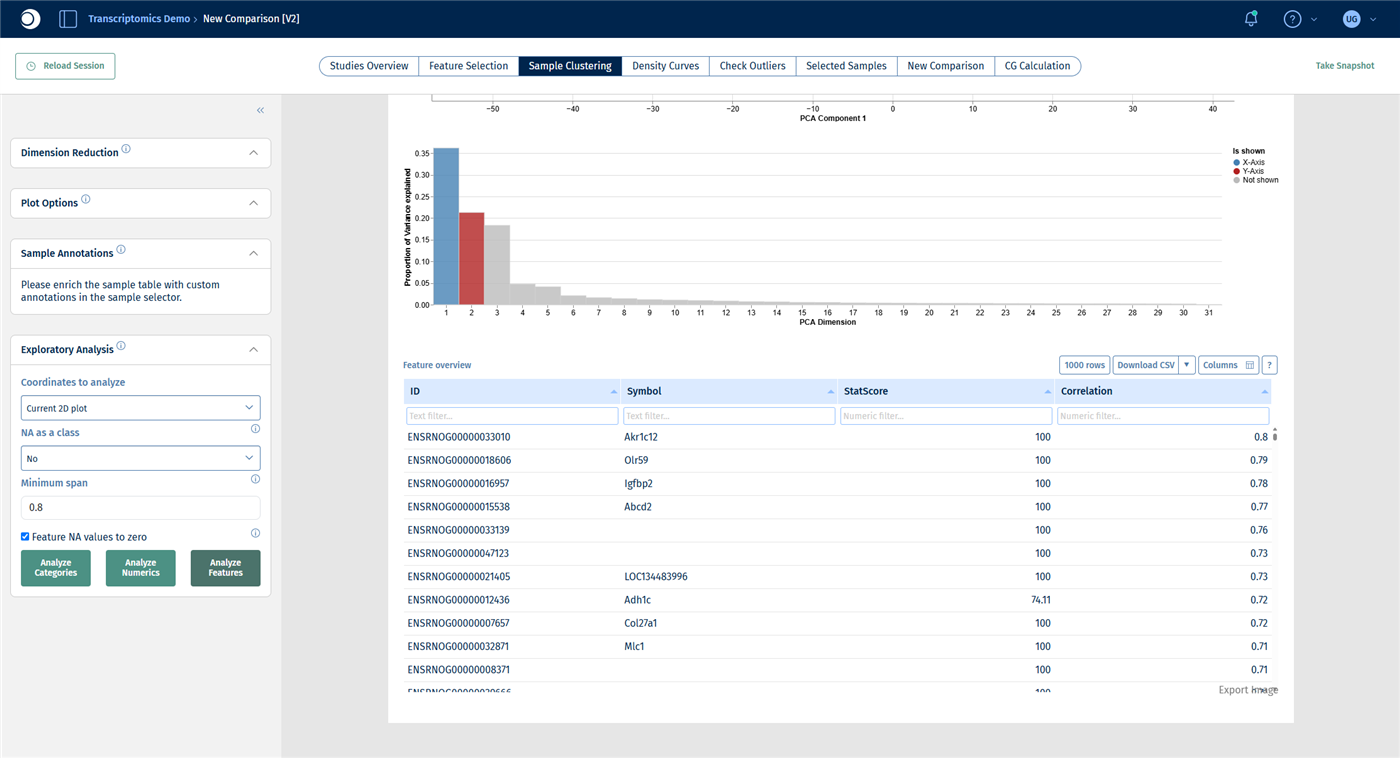
The top genes include Akr1c12, Igfbp2, Abcd2 and Adh1c.
Step 6: Find the biology behind the driving genes
A list of top genes is hard to interpret on its own. An over-representation analysis tells you which pathways and processes are enriched among them. The Enrichment Visualization app accepts any gene list, not only the results of a comparison.
- Note the gene symbols of the top 50 genes from the feature table of step 5.
- Open the Enrichment Visualization app from the start page.
- Under Data selection, set the data source to Manual input, Species to Rn and Type to Genesymbol.
- Open the Up-regulated block by clicking its title, select Manual Freetext and paste the gene symbols, one per line. Set Type to Gene and Species to Rn, then click Apply.
- Under Gene set collections, check GO BP, Wikipathways (Hs) and Wikipathways (Rn).
- Click Perform Enrichment Analysis. The calculation takes a few minutes.
Note: The species must be set twice: once for the whole input and once for the gene list itself.
The results are shown in the same tabs as for a comparison; see Enrichment Visualization and step 5 of the guide From differential expression to pathway enrichment.
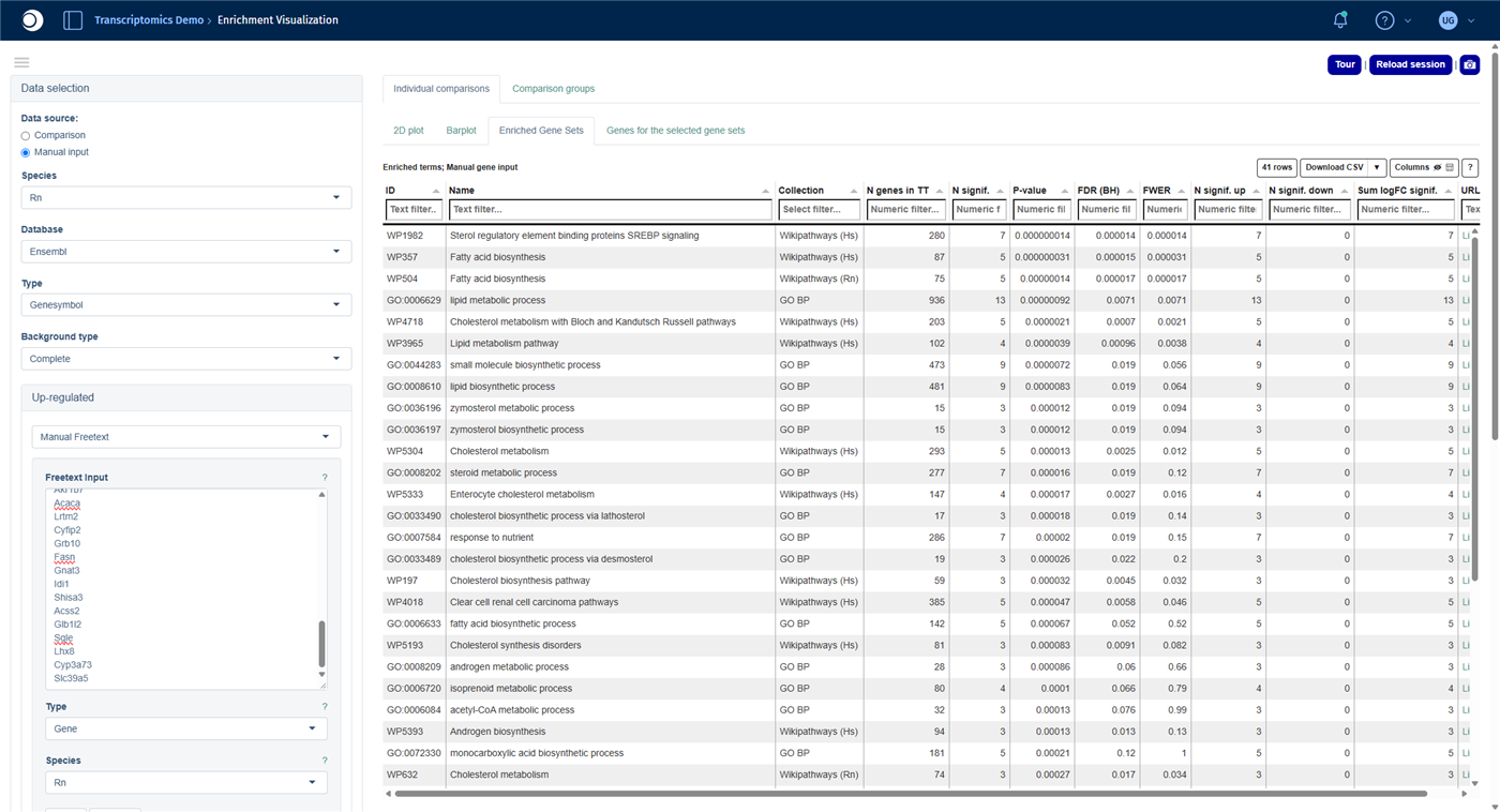
Check your result: gene list
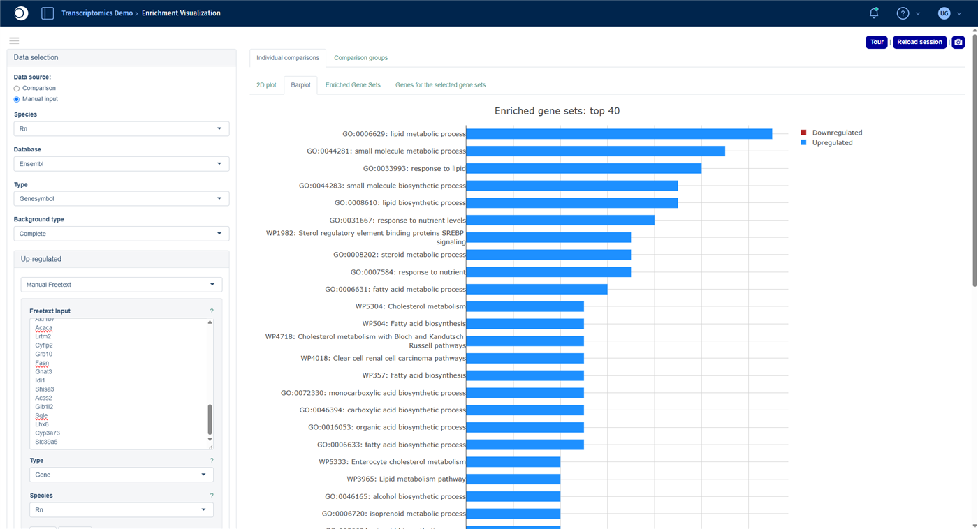
Check your result: enriched gene sets
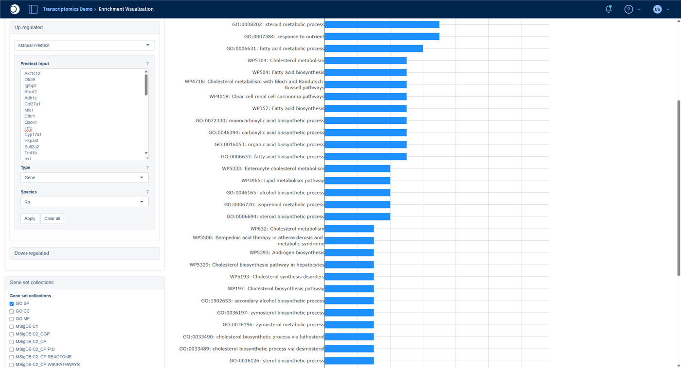
About 40 gene sets are enriched. The top hits are SREBP signaling, Fatty acid biosynthesis, Cholesterol metabolism with Bloch and Kandutsch-Russell pathways and the GO term lipid metabolic process. The genes that separate young from old and female from male liver samples are dominated by lipid, fatty acid and cholesterol biosynthesis.
Troubleshooting
I cannot see the Exploratory Analysis panel.
The panel is the last one in the left sidebar. Collapse the panels above it, for example Dimension Reduction and Plot Options, by clicking their headers.Analyze Features does not react.
After closing a message window, the first click on the button is sometimes ignored. Click it a second time.The Enrichment Visualization finds no or only a few gene sets.
Check that the species is set to your organism in both places (step 6) and that the gene symbols are spelled as in PanHunter. Add the human collections, for example Wikipathways (Hs): they are more comprehensive, and PanHunter maps your genes to their human orthologs.Next steps
3 - From single-cell data to cell-type-specific differential expression
Explore a single-cell study, aggregate it into a pseudobulk study, compare disease and control in every cell type at once and find the pathways that change in each cell type.
Single-cell and single-nucleus RNA-seq show the expression of every cell, but a single cell contains few reads, and cells from the same person are not independent replicates. To compare disease and control, a robust approach is to sum up the cells of each cell type per donor into one pseudobulk profile and to compare these profiles with the methods used for bulk RNA-seq.
This guide walks you through this approach. You will:
- explore a single-cell study and its cell types in the scExplorer app,
- create a pseudobulk study with one profile per donor and cell type,
- calculate a disease-versus-control comparison for every cell type in one run,
- find out which cell types respond most strongly,
- compare pathway enrichment across all cell types in a heatmap and
- look at one pathway in one cell type.
The guide takes about 45 minutes, most of it waiting for calculations.
Before you start
- Access: You need access to a PanHunter project with single-cell data and the apps scExplorer, New Comparison [v2], Comparisons, Enrichment Visualization and Pathway Mapping, and permission to calculate comparisons.
- Example data: The guide uses the study Hs_Heart_KoenigSn2022, a public single-nucleus RNA-seq study of human hearts by Koenig et al. (2022, Nature Cardiovascular Research). It contains about 220,000 nuclei from 25 healthy donor hearts and 13 hearts with dilated cardiomyopathy (DCM), annotated with 15 cell types. If your project does not contain this study, follow the same steps with your own single-cell study.
- Background: For the statistics of the comparison, see Differential gene expression analysis. The guide From differential expression to pathway enrichment explains the comparison set-up and the enrichment analysis for a single comparison in more detail.
Step 1: Explore the cell types
- Open the scExplorer app from the start page of your project.
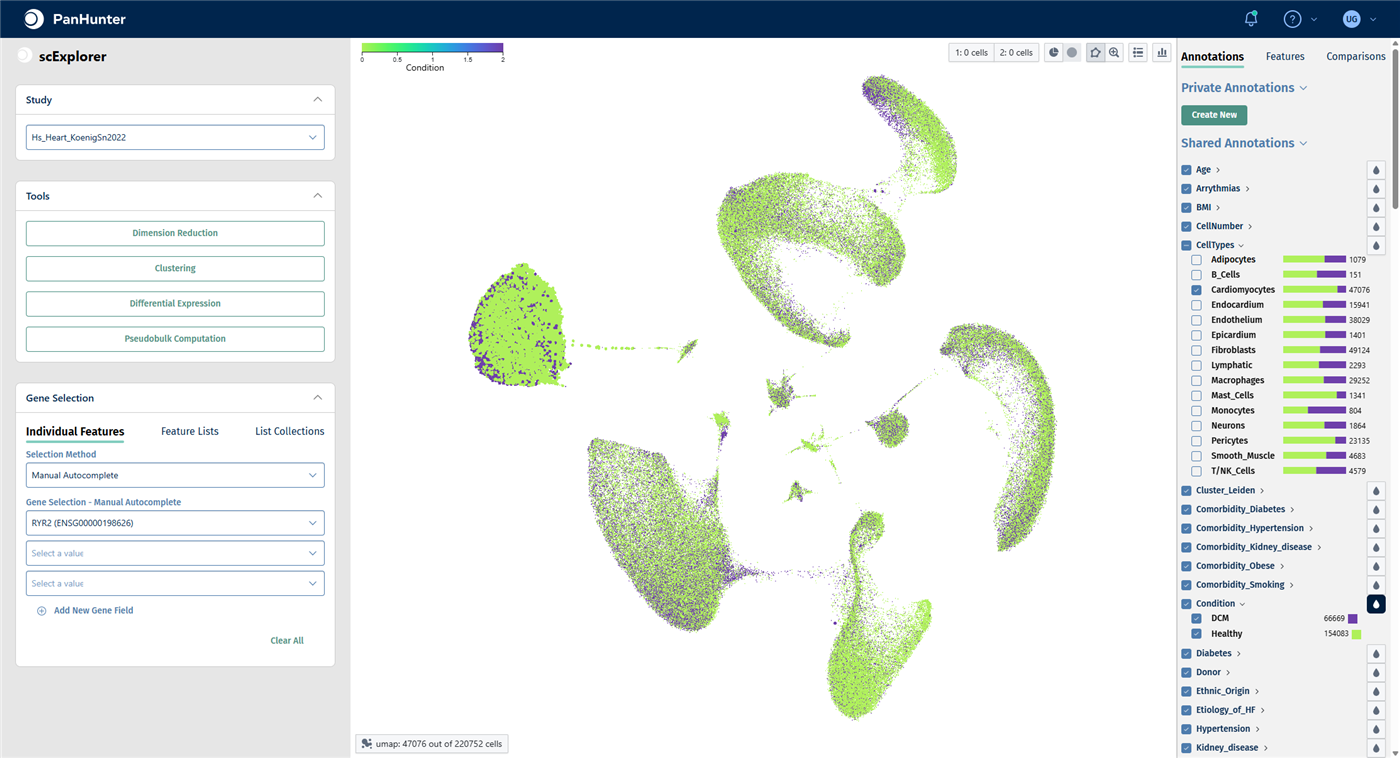
- In the Study panel, select Hs_Heart_KoenigSn2022. The cells are shown in a UMAP embedding.
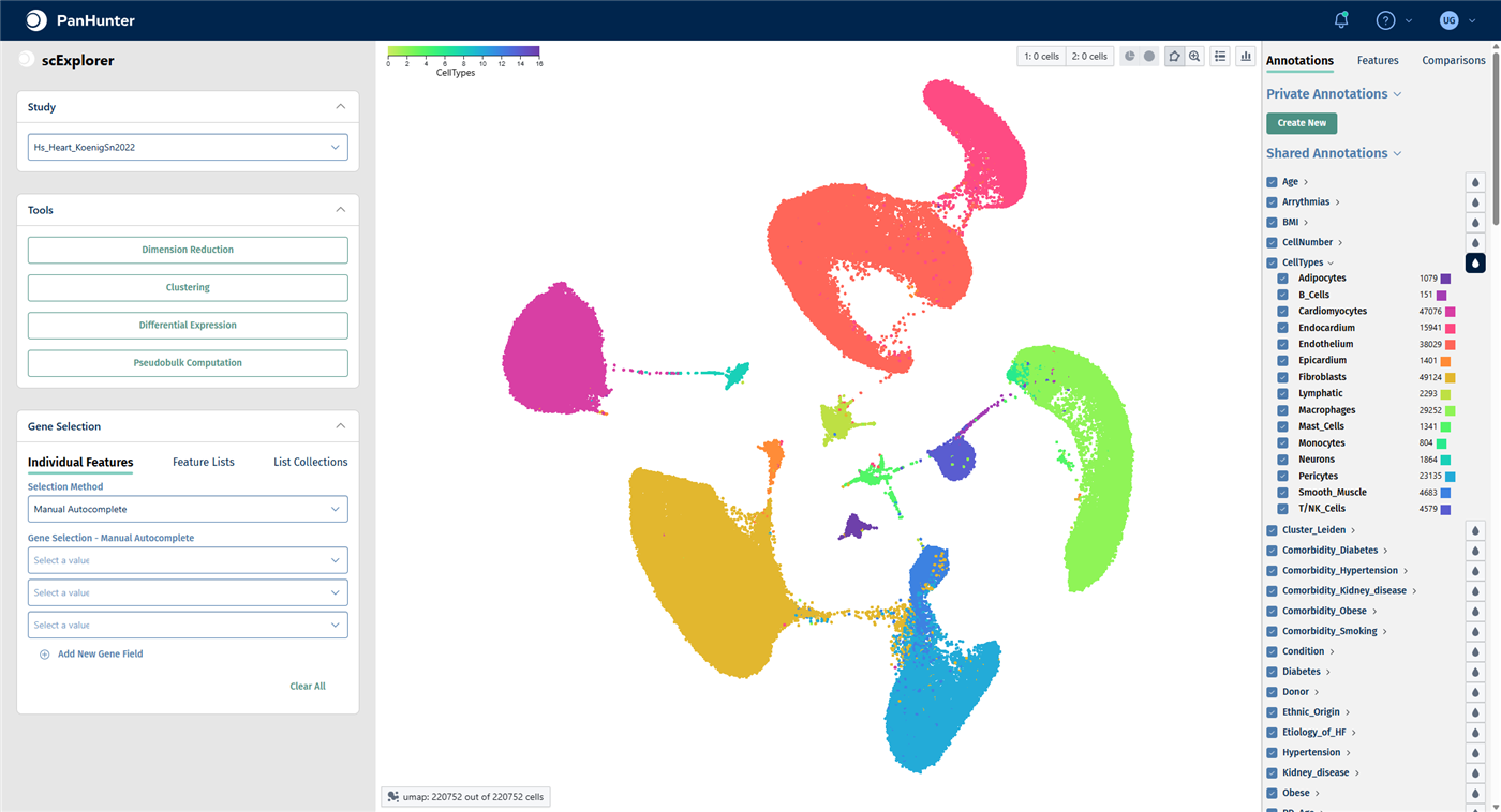
- In the right-hand panel, open the Annotations tab. Under Shared Annotations, click the droplet icon next to CellTypes to color the cells by cell type. Click the arrow next to CellTypes to see the list of cell types with their number of cells.
For all functions of the app, see scExplorer.
Check your result
The plot reads umap: 220752 out of 220752 cells. The 15 cell types form separate clusters; the largest populations are fibroblasts, cardiomyocytes, endothelium and macrophages.
Marker genes confirm that a cluster really is the cell type it is labeled as:
- In the Gene Selection panel on the left, click the first field under Gene Selection - Manual Autocomplete, type
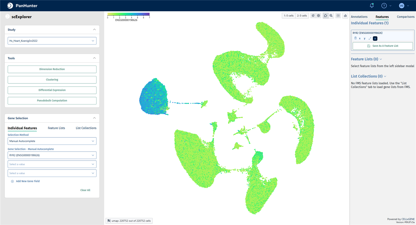
RYR2 and select RYR2. RYR2 is a calcium channel typical of cardiomyocytes. - The right-hand panel switches to the Features tab. Click the droplet icon below the gene to color the cells by its expression.
Check your result: marker gene
Only the cardiomyocyte cluster shows high RYR2 expression.
To see how disease and control cells are distributed within a cell type:
- In the Annotations tab, uncheck the box of CellTypes to deselect all cells, then check Cardiomyocytes only.
- Click the droplet icon next to Condition. The two conditions are called DCM and Healthy.
- Check the box of CellTypes again to select all cells before you continue.
Check your result: cardiomyocytes by condition
47,076 cardiomyocytes are selected; all other cells are greyed out. The bars next to each cell type show the proportion of DCM and healthy cells.
Step 2: Create a pseudobulk study
A pseudobulk study sums up the counts of all cells that share the same values in the aggregation keys. With the keys SampleID and CellTypes, you get one profile per donor sample and cell type.
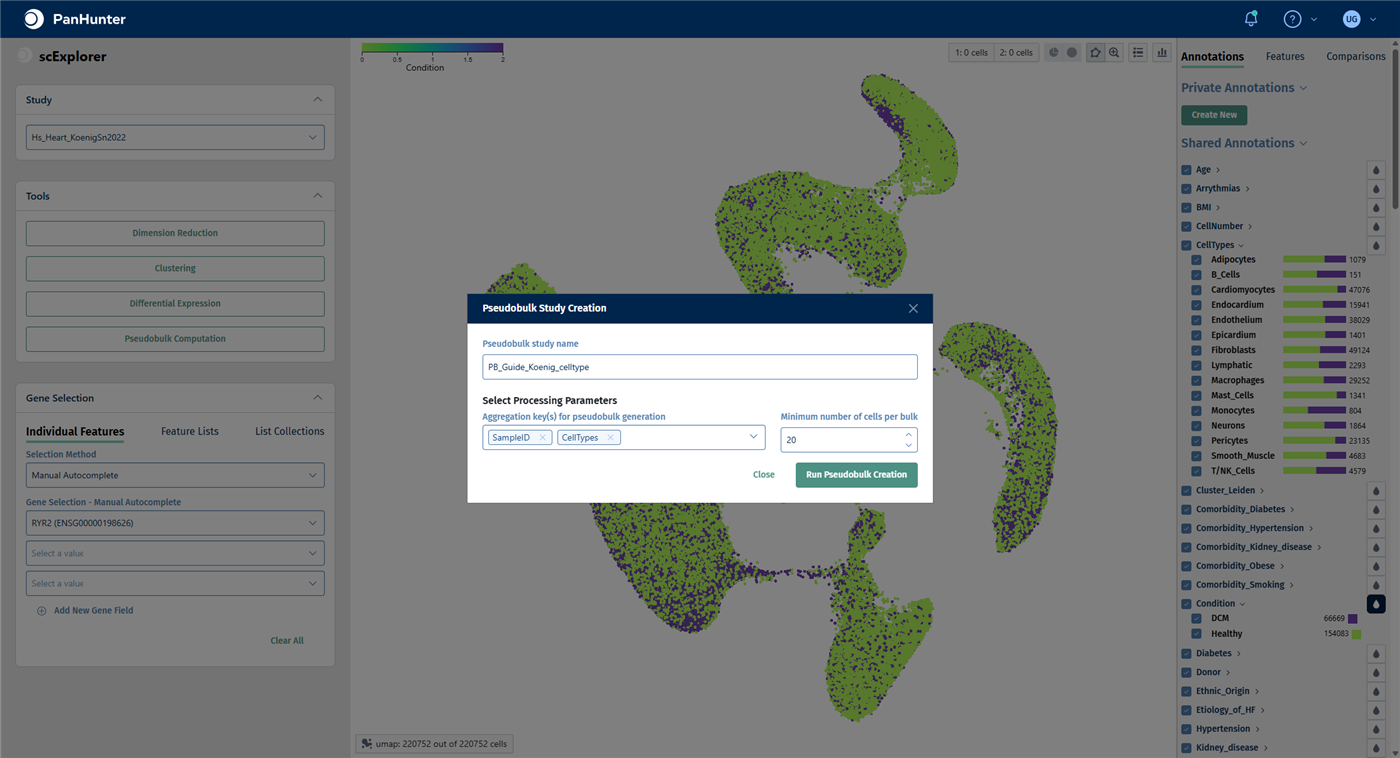
- In the Tools panel on the left, click Pseudobulk Computation. The Pseudobulk Study Creation window opens.
- Enter a Pseudobulk study name, for example
PB_Koenig_celltypes. Pseudobulk studies usually start with PB_. - In Aggregation key(s) for pseudobulk generation, keep SampleID and add CellTypes.
- Keep Minimum number of cells per bulk at 20. Profiles built from fewer cells are left out because they are too noisy.
- Make sure that all cells are selected, then click Run Pseudobulk Creation.
Check your result
When the calculation has finished, the pseudobulk study is available as a normal study in the Sample Selector of the other apps. No further approval step is needed.
Note: The project used in this guide already contains a pseudobulk study with the same design, PB_Hs_Heart_KoenigSn2022_celltype. The following steps and screenshots use it. If you created your own, select your study instead.
Step 3: Check the pseudobulk study
- Open the New Comparison [v2] app from the start page.
- In the Sample Selector, start typing the name of the pseudobulk study in Studies and select it.
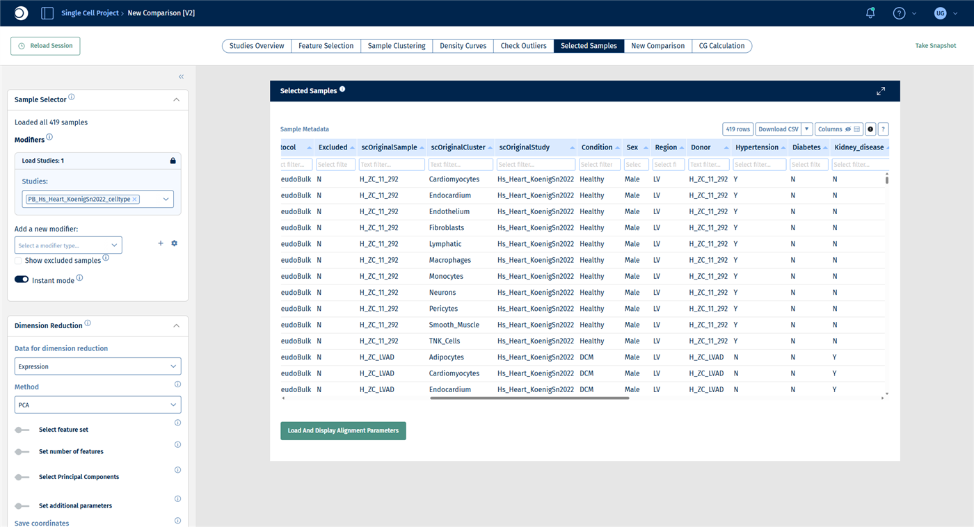
- Open the Selected Samples tab and look at the sample table.
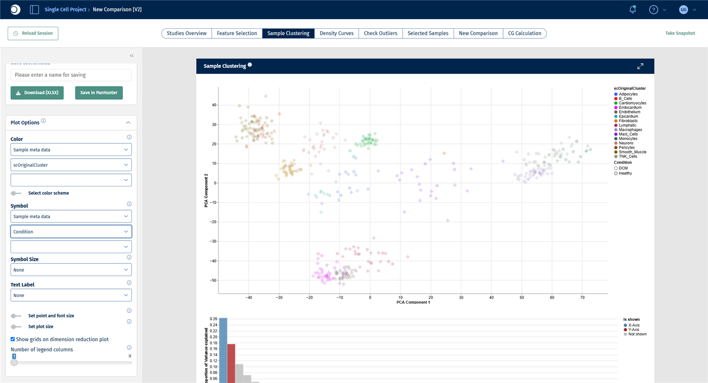
- Open the Sample Clustering tab. In Plot Options, set Color to Sample meta data and scOriginalCluster, and Symbol to Sample meta data and Condition.
Important: In the pseudobulk study, the cell type is stored in the column scOriginalCluster and the donor sample in scOriginalSample, not under the names used in scExplorer. All other metadata, such as Condition, Sex and Age, keep their names.
Check your result: samples
The study contains 419 samples: one pseudobulk profile for each combination of donor sample and cell type that had at least 20 cells.
Check your result: PCA
The profiles cluster by cell type. The differences between DCM and healthy samples are much smaller than the differences between cell types, which is why each cell type gets its own comparison in the next step.
Step 4: Compare DCM and healthy hearts in every cell type
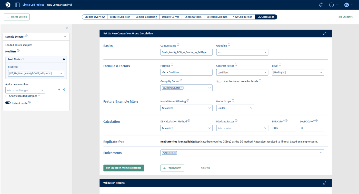
With a Group By Factor, a single comparison group calculation creates one comparison per level of that factor, here one per cell type. For a description of all fields, see New Comparison: CG Calculation.
- Open the CG Calculation tab.
- Under Basics, enter a CG Run Name, for example
Koenig_DCM_vs_Healthy_by_CellType, and keep Grouping at n:1. - Under Formula & Factors:
- enter the Formula
~Sex + Condition, so that the model accounts for differences between women and men. - set Contrast Factor to Condition and Level to Healthy. Healthy is the reference; DCM is compared against it.
- set Group By Factor to scOriginalCluster.
- Leave all other sections at their defaults.
- Click Run Validation And Create Recipes.
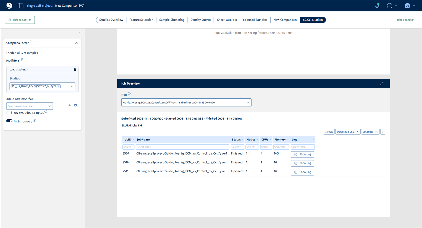
- Check the validation results, then click Submit Calculation To SLURM and follow the progress in the Job Overview.
Check your result: set-up
Check your result: validation
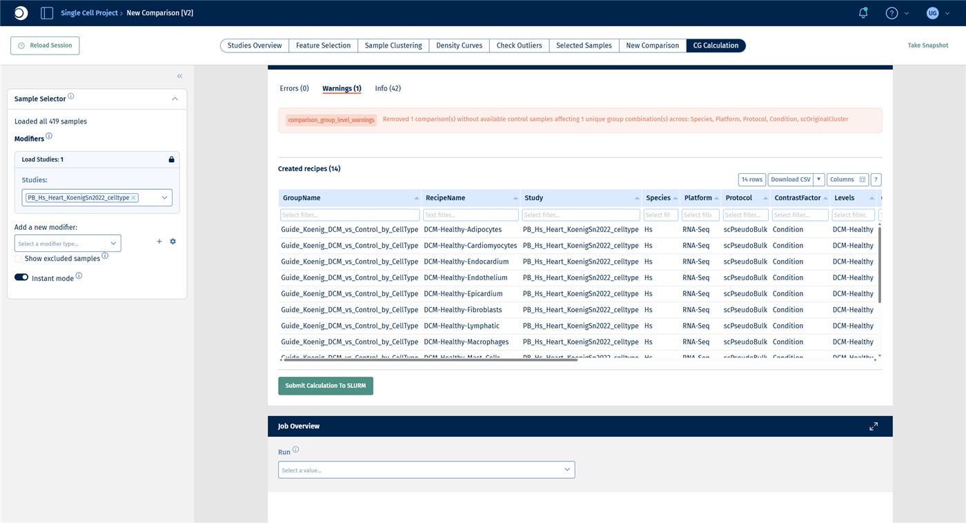
- Errors (0).
- Warnings (1): one comparison was removed because no control samples are available. This is the cell type B_Cells, which occurs only in DCM samples.
- Created recipes (14): one recipe DCM-Healthy-<cell type> per remaining cell type. The table shows the number of DCM and healthy samples per recipe. Cell types with only a few samples, such as Epicardium with 2 DCM samples, give less reliable results.
- The DE method is autoselected as deseq2.
Check your result: job overview
For this example the run takes about six minutes. The Job Overview does not refresh by itself: reload the page and select the run again to update the status.
Step 5: Find the cell types that respond
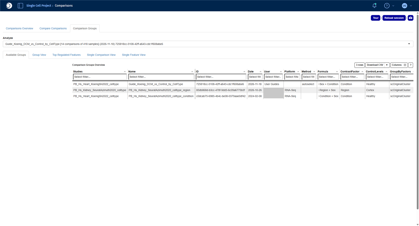
- Open the Comparisons app from the start page and open the Comparison Groups tab.
- In Analyze, select your run. It is listed with the number of comparisons and samples.
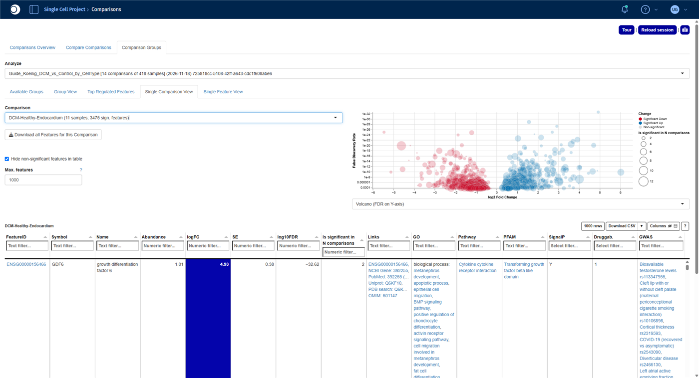
- Open the Single Comparison View tab. The Comparison list shows the number of significant features for each cell type. Select DCM-Healthy-Endocardium.
For all functions of the app, see Comparisons.
Check your result: comparison group
Check your result: significant features per cell type
The number of significant features differs a lot between cell types:
| Cell type | Significant features |
|---|
| Fibroblasts | 5313 |
| Cardiomyocytes | 5013 |
| Endothelium | 3632 |
| Endocardium | 3475 |
| Macrophages | 3423 |
| Pericytes | 2766 |
| Smooth_Muscle | 484 |
| Neurons | 248 |
| TNK_Cells | 110 |
| Epicardium | 109 |
| Lymphatic | 78 |
| Adipocytes | 47 |
| Mast_Cells | 8 |
| Monocytes | 0 |
Fibroblasts, cardiomyocytes and the cells lining the vessels and heart chambers (endothelium, endocardium) respond most strongly to the disease. Part of the differences also reflects sample size: small populations have fewer profiles and therefore less statistical power.
Check your result: endocardium
The comparison reads DCM-Healthy-Endocardium (11 samples; 3475 sign. features). The gene with the lowest FDR is GDF6, upregulated in DCM.
Step 6: Compare pathways across all cell types
The Comparison groups tab of the Enrichment Visualization app shows the enrichment results of many comparisons side by side in one heatmap.
- Open the Enrichment Visualization app from the start page and open the Comparison groups tab.
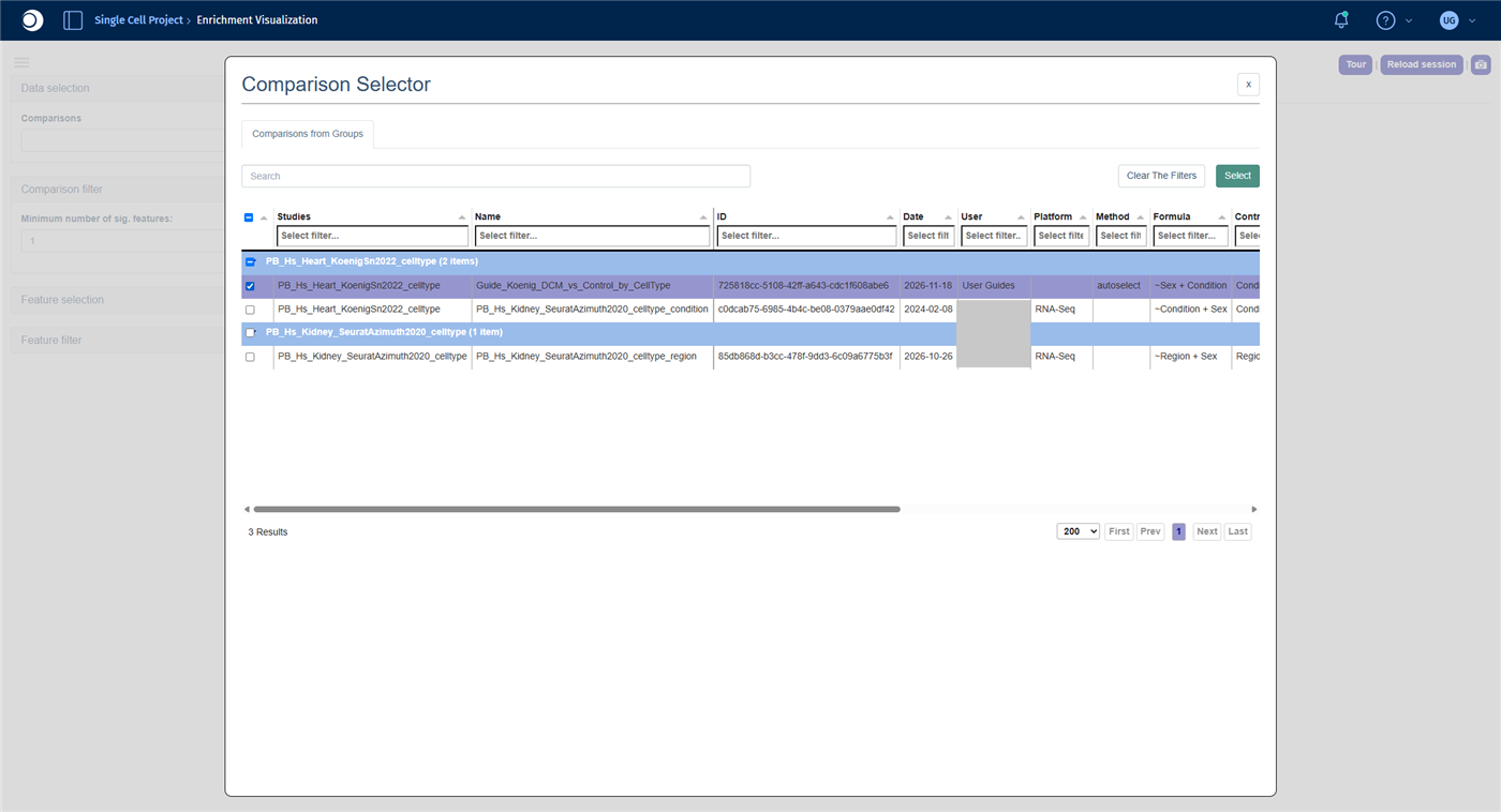
- Under Data selection, click into the Comparisons field. In the Comparison Selector, check your run and click Select. In the next view, check the box in the header row to select all comparisons and click Select again.
- Open Feature selection, set Heatmap Y-axis levels to Feature list collections and select the collection Wikipathways. The analysis method switches to Fisher.
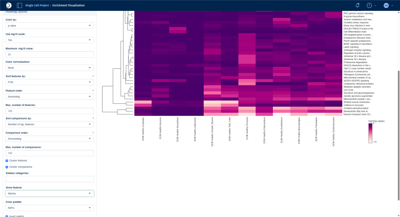
- Open Heatmap options and set Show feature to Names, so that the rows show pathway names instead of IDs.
Comparisons with too few significant features, here Monocytes and Mast_Cells, are left out.
Check your result: Comparison Selector
Check your result: heatmap
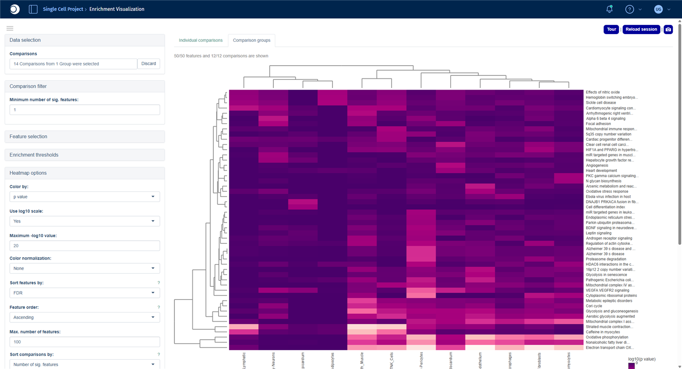
The heatmap shows the 50 most significant pathways (rows) across the cell types (columns); the darker the color, the lower the p-value. Both axes are clustered, so cell types with similar pathway changes are placed next to each other.
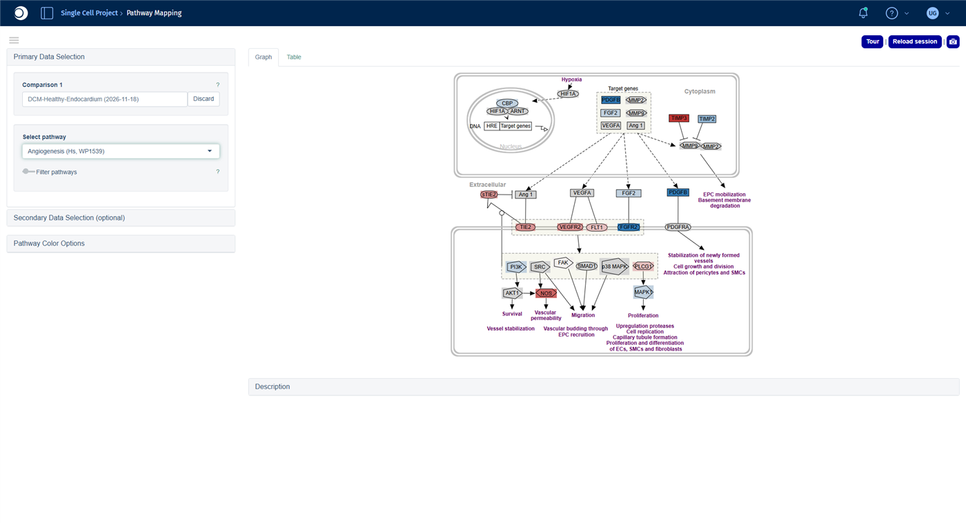
- The strongest signals are energy metabolism pathways such as Electron transport chain (OXPHOS), Oxidative phosphorylation and Glycolysis and gluconeogenesis, mainly in endothelium, fibroblasts and pericytes.
- Angiogenesis (WP1539) is enriched almost only in the endocardium. VEGFA VEGFR2 signaling is enriched in the endocardium and in pericytes.
Hover over a cell of the heatmap to see the full pathway name and the p-value; long names are cut off on the axis. Angiogenesis in the endocardium is the starting point for the next step.
Check your result: heatmap options
Step 7: Look at a pathway in one cell type
- Open the Pathway Mapping app from the start page.
- Click into Comparison 1. In the Comparison Selector, open Comparisons from Groups, check your run and click Select. Type
Endocardium into the filter of the Name column, press Enter, check the comparison and click Select. - In Select pathway, type
Angiogenesis and select Angiogenesis (Hs, WP1539).
For coloring options and the table view, see Pathway Visualization.
Check your result
Blue genes are upregulated, red genes downregulated in the endocardium of DCM hearts. The growth factor PDGFB and the receptor FGFR2 are up, while the receptors VEGFR2 and TIE2 and the nitric oxide synthase NOS are down: a pattern that points to disturbed formation and maintenance of blood vessels.
Troubleshooting
My pseudobulk study does not appear in the Sample Selector.
The creation runs in the background and can take a while for large studies. Reload the app after some minutes. If the study still does not appear, contact your PanHunter administrator.The validation removes comparisons.
A comparison needs samples of both conditions. Cell types that occur in only one condition, or whose profiles were dropped because of the minimum number of cells, are removed with a warning. The remaining comparisons are calculated normally.I cannot find the column CellTypes in New Comparison [v2].
In pseudobulk studies, the cell type is stored in the column scOriginalCluster and the donor sample in scOriginalSample.Next steps